https://doi.org/10.5194/nhess-17-1375-2017 © Author(s) 2017. This work is distributed under the Creative Commons Attribution 3.0 License.
A novel method of sensitivity analysis testing by applying the
DRASTIC and fuzzy optimization methods to assess groundwater
vulnerability to pollution: the case of the Senegal River basin in Mali
Keita Souleymane1,2and Tang Zhonghua1
1Department of Hydrology and Water Resources, School of Environmental Studies of China University of Geosciences, Lumo Road, Wuhan 430074, China
2Department of Civil Engineering, ENI-ABT, 410, Av. Van Vollenhoven P.O. Box, 242 Bamako, Mali Correspondence to:Keita Souleymane ([email protected])
Received: 27 March 2017 – Discussion started: 3 April 2017 Accepted: 4 July 2017 – Published: 9 August 2017
Abstract. Vulnerability to groundwater pollution in the Senegal River basin was studied by two different but com-plementary methods: the DRASTIC method (which evalu-ates the intrinsic vulnerability) and the fuzzy method (which assesses the specific vulnerability by taking into account the continuity of the parameters). The validation of this applica-tion has been tested by comparing the connecapplica-tion in ground-water and distribution of different established classes of vul-nerabilities as well as the nitrate distribution in the study area. Three vulnerability classes (low, medium and high) have been identified by both the DRASTIC method and the fuzzy method (between which the normalized model was used). An integrated analysis reveals that high classes with 14.64 % (for the DRASTIC method), 21.68 % (for the normalized DRAS-TIC method) and 18.92 % (for the fuzzy method) are not the most dominant. In addition, a new method for sensitivity analysis was used to identify (and confirm) the main param-eters which impact the vulnerability to pollution with fuzzy membership. The results showed that the vadose zone is the main parameter which impacts groundwater vulnerability to pollution while net recharge contributes least to pollution in the study area. It was also found that the fuzzy method better assesses the vulnerability to pollution with a coincidence rate of 81.13 % versus that of 77.35 % for the DRASTIC method. These results serve as a guide for policymakers to identify areas sensitive to pollution before such sites are used for so-cioeconomic infrastructures.
1 Introduction
A key component to building a territory is the vulnerabil-ity map, which is a fundamental water qualvulnerabil-ity assessment that aids the development of underground water resources. Among the myriad of functions delivered by a geographic information system (GIS), its capability for multi-criteria analysis is essential for developing vulnerability maps for an aquifer system. Water quality information is a basic data requirement for implementing any water management deci-sion. It provides necessary information for assessing risk of groundwater pollution and remediation measures needed to control future pollution levels. This information can be re-trieved from groundwater pollution vulnerability maps. To assess the vulnerability of groundwater to pollution, 24 meth-ods exist, which can be classified into three groups.
– Comparison methods are used mainly for very large study areas and take into consideration two to three pa-rameters.
– Methods of analog relationship and numerical models are based on simple or complex mathematical laws and are recommended for assessing the vulnerability of ra-dioactive sites.
– Parametric systems are composed of three subsystems: – The matrix system, adapted for local use, is based
– The class system defines a range for each parame-ter considered necessary for assessing vulnerability, then subdivides each of the intervals selected based on the variability of the parameter. The final score resulting from the summation (or multiplication) of each score for the different parameters should be divided by the number of classes chosen.
– The weighted class system is based on assigning ratings to the parameters, which are retained as nec-essary for the evaluation of groundwater vulnera-bility by defining intervals, as is the case with other methods cited previously. Subsequently a weight is applied for each parameter according to its impor-tance to the assessment of vulnerability.
Water is one of the most essential parts of our daily life. Wa-ter management is becoming increasingly problematic due to, for example, climate, pollution and environmental issues. Surface water and groundwater are often polluted. Since the water system is a cycle, water in the air, water on land and water underground are all connected. Groundwater and sur-face water are connected through a very complicated hy-drogeological system that can lead to mutual contamination, which means that if groundwater is polluted it can affect the upper surface water and if surface water is polluted it can affect the underlying groundwater.
Sustainable management of Senegal River basin resources is a major issue for the four riparian countries of Guinea, Mali, Mauritania and Senegal.
The multiple uses of water and the multinational nature of the basin led the riparian countries to create the Organization for the Development of the Senegal River (OMVS in French) to manage the basin’s water resources. For this, each country needs data and information enabling it to monitor and pre-dict the evolution of the resources, in particular in light of the importance of climate variability in the region marked by the recurrence of drought, the potential impacts of climate change and the increasing impacts of population on water re-sources. Many other water uses in the basin also require data and information for their activities.
The Senegal River basin in Mali is increasingly dominated by cultures and industries that use chemicals. This strong de-mand for chemicals threatens the quality of groundwater re-sources. Groundwater reserves are substantial and are being used to cover different needs. They are also used as a source of drinking water in the region, which is experiencing rapid population growth at a rate of 3 % per year (O.M.V.S., 2013). The quality of this groundwater resource is constantly put to the test because of the growth of both point and diffuse pollu-tion sources. To prevent the risk of pollupollu-tion of groundwater, a modified approach is the gathering of knowledge about ar-eas vulnerable to pollution. Civita (1994) showed that aquifer groundwater’s changes (in quality and quantity) in time and space are due to natural processes and/or human activities.
Work already done in the area (Newton, 2007; UNESCO, 2012) mainly concerns the quantity of water resource man-agement. Other studies (Anoh, 2009; Jourda et al., 2007) have focused on the quality of water resources but they did not focus on the same area nor did they find vulnerability zones.
However, none of these studies have investigated the im-pact of human and natural activities on groundwater re-sources in the basin of the Senegal River in Mali. Thus, the present study uses fuzzy and DRASTIC methods to evaluate the intrinsic and specific vulnerability to pollution to high-light those impacts. The intrinsic vulnerability method is in-flexible because its weights and ratings are fixed according to hydrogeological parameters, while the specific vulnerability method is flexible and takes into account local hydrogeolog-ical conditions and continuity of parameters (Afshar et al., 2007; Antonakos et al., 2007; Alemi-Ardakani et al., 2016; Madhumita et al., 2016).
The DRASTIC method is the most common method to assess groundwater vulnerability to pollution (Denny et al., 2007; Bojórquez-Tapia et al., 2009; Dhar et al., 2014). How-ever, this method is increasingly criticized for the choice of hydrogeological features; the weights and the ratings do not necessarily agree with the reality of the study area and its specificity (Denny et al., 2007; Dhar et al., 2013; Madhumita et al., 2016). So to improve and adapt the DRASTIC model to the particularity of the study area, it is better to modify the classical model or combine it with other developed models to get better results. Many studies proposed methods which combined DRASTIC and other methods (Yu et al., 2012; Dhar and Patil, 2012; Fernando et al., 2013; Madhumita et al., 2016). Leone et al. (2009), Luis et al. (2009) and Ne-shat et al. (2015a, b) all proposed modified models to as-sess groundwater vulnerability to pollution. However, none of them focused on a comparison between classical sensitiv-ity analyses (single parameter and map removal) and fuzzy membership. The DRASTIC method is essentially based on subjective setting of study area hydrogeological conditions (Nobre et al., 2007; Madhumita et al., 2016) while the fuzzy concept is based on membership, which is an objective set-ting of study area hydrogeological conditions (Pacheco et al., 2015; Madhumita et al., 2016). For example, member-ship expresses the relations between two given parameters and also the degree of truth or falseness of these relations (Pacheco et al., 2015; Madhumita et al., 2016). This tech-nique has been used by many authors – such as Pacheco et al. (2015), Madhumita et al. (2016), Pathak et al. (2009), Sahoo et al. (2016a, b), Saidi et al. (2011) and Sener et al. (2013) – but most of these studies assessed pollution risk (Pacheco and Van der Weijden, 2011, 2012) and did not com-pare intrinsic with specific vulnerability or different types of sensitivity analyses with memberships to identify parameter impact on groundwater vulnerability to pollution.
of risks of pollution of groundwater resources in this area through sustainable management.
The DRASTIC method uses weighted classes and was de-veloped by the US Environmental Protection Agency (EPA) and the National Water Well Association (NWWA) in 1987 to evaluate the vulnerability of groundwater to pollution. Al-though it was not originally designed for GIS, it is a classic spatial analysis widely used in GIS.
The objective of DRASTIC is to give a standard method-ology that gives reliable results useful for efforts to protect groundwater.
DRASTIC generates an index, or “score”, for the potential pollution of groundwater resources. This index covers the en-tire range from 23 to 226. Note that the vulnerability to pol-lution is higher for higher notes.
The DRASTIC method uses seven hydrological parame-ters: the depth of the water level of the water table (D), the net recharge (R), the lithology of the aquifer (A), the soil tex-ture (S), the topography slope of the field (T), the impact of the unsaturated zone (I) and, finally, the hydraulic conductiv-ity or permeabilconductiv-ity of the saturated zone (C).
In GIS, each parameter is scored on a layer by assigning a weight coefficient corresponding to the parameter, i.e., its in-fluence on the vulnerability of the aquifer. Then these layers are superimposed on a layer for which results will be calcu-lated as the DRASTIC pollution index (DPI). The layers will have the same cartographic features – a single projection sys-tem, identical units of length, identical geographical area and the same resolution – because this system uses a matrix for-mat for all calculations.
DPI is dimensionless. The number or the order of magni-tude has no meaning in itself. The unity of the DPI occurs when comparing two sites or one site to several other sites. The site with the highest DPI will be considered most sus-ceptible to contamination or pollution.
More than 24 vulnerability assessment methods of ground-water to pollution are identified in the literature. The method most often used is the DRASTIC method. It was developed by Aller et al. (1987) and is an assessment method (vulnera-bility aquifers) based on weights and ratings for different pa-rameters (generally between 1 and 10). A weight is also allo-cated according to the relative importance of each of the pa-rameters used. The DRASTIC numerical rating system incor-porates seven different physical parameters involved in the transportation process and mitigation of contaminants: water depth, effective recharge, aquifer and soil type, topography, impact of unsaturated zone and hydraulic conductivity. In the first step, a numerical value ranging from 1 to 5 is allocated to each of the seven parameters, topography, vadose zone and hydraulic conductivity of aquifer media. Each of these pa-rameters is a weight (predetermined value), between 1 and 5, that reflects the importance of the parameter in the transport processes and contaminant attenuation. A key parameter is assigned a weight of 5 while a setting with less impact on the fate of a contaminant is assigned a weight of 1. In the
second step, each of the seven parameters is assigned a value ranging from 1 to 10, defined in terms of ranges of values. The smallest value represents lower vulnerability to contam-ination (Dc,Rc,Ac, etc.). For each hydrogeological unit, the seven parameters must then be evaluated to give each a rating that can vary from 1 to 10. A rating of 1 corresponds to the lowest vulnerability while a rating of 10 reflects the condi-tions most likely to be contaminated. DRASTIC’s parameters were reclassified in ArcMap and assigned a score based on rankings ranging from 1 to 10 and a weighting to help merge factors together in the DRASTIC equation in GIS. Each of the seven parameters was then assigned a multiplicative fac-tor (w) ranging from a value of 5 for the most significant factors to 1 for factors that are less so.
The DPI was determined according to Eq. (1) as in Os-born et al. (1998), whereD,R, A,S,T,I andC are the seven parameters of the DRASTIC method,wis the weight of the parameter andr the associated rating. The weights of the parameters of the DRASTIC method used (Table 1) are those defined by Aller et al. (1987). The reference values of the index used in DRASTIC are those provided by Engel et al. (1996) and represent the measurement of the hydrogeo-logical aquifer vulnerability.
DPI=DrDw+RrRw+ArAw
+SrSw+TrTw+IrIw+CrCw (1)
or
DPI=X7
k=1rkwk, (2)
whereris the rating (1 to 10),wis the weight (1 to 5) andk
is the parameter (1 to 7).
In the final step, the calculation of the DRASTIC index for each hydrogeological unit is obtained by multiplying the rat-ing of each parameter by it correspondrat-ing weight. DPI repre-sents the level of risk of the aquifer unit to be contaminated. It can reach a maximum of 226 (100 %) and a minimum value of 23 (0 %).
2 Materials and methods
total area of 289 000 km2. Along 760 km, Bafing rises at an altitude of 800 m in the Fouta Djallon in Guinea and flows north across the plates of the Sudanese region before reach-ing Bafoulabé. It brreach-ings more than half of the total flow of the Senegal River with 430 m3s−1 mean annual flow. The river is characterized by the presence of falls and rapids. With a length of 560 km, Bakoye’s source is near the southern boundary of Mandingo Mountain in Guinea, at an altitude of 706 m. At its confluence with Bafing, Bakoye has a mean annual flow of 170 m3s−1. This river also passes a relatively large number of small waterfalls and rapids. Bafoulabé is lo-cated downstream on the right bank; the main tributaries of the Senegal River are Kolombiné, Karakoro and Gorgol. On the left bank, Falémé River is the largest tributary at 650 km long; it rises in the northern part of Fouta Djallon, at an al-titude of 800 m. It joins the Senegal River 30 km upstream from Bakel. The annual flow at its outlet in the Senegal River is about 200 m3s−1.
With a length of 1800 km, Senegal River starts in north-ern Guinea, crosses the westnorth-ern part of Mali and remains the borderline between the territories of the Republic of Senegal and the Islamic Republic of Mauritania.
There are two main parts:
– the Senegal upper basin is located upstream of Bakel, a mountainous region, and is made up of the basins of the Falémé, the Bafing, the Bakoye and Baoulé rivers; – the Senegal lower basin is located downstream of Bakel
in a very flat, slightly accentuated area, where the maxi-mum does not exceed 400 m (Massif Assaba) and where the river flows in the middle of a very wide valley; – the watershed of the river covers a total area of
289 000 km2 with 155 000 km2 in Mali (upper basin), spread between Kayes (Kéniéba, Bafoulabé, Kita, Kayes, Diéma, Yélimané and Nioro) and Koulikoro (Banamba, Kolokani and Nara).
Our study concerns the upper Senegal basin (Fig. 1a), which is situated in Mali.
The working material consists of multiple data sources. This includes piezometric data from filed measurements of groundwater level collected in different years in the region and complemented by the database “sigma” of the National Water Directorate (DNH). Drilling data sheets were provided by various campaigns monitoring the supply of drinking wa-ter; also, the National Water Laboratory (LNE) allowed the use of drilling depth data, groundwater levels, lithological cuts and pumping test. These data helped create several vul-nerability maps. To these data we added geological maps of the region and the soil sketch of Mali provided by the FAO.
Finally, the coordinates of the Shuttle Radar Topography Mission (SRTM) (http://srtm.csi.cgiar.org) were used for the land use and land cover images of the study area. This im-age treatment was used to establish a digital elevation model
(DEM) with a resolution of 90 m and highlights the slope map.
The processing of these data is performed on ArcGIS 10.0 for cartographic processing, processing of satellite images and generating the slope map and the combination of other thematic maps.
For this study we used two different methods: one to assess the intrinsic vulnerability (DRASTIC) and the second to find the specific vulnerability (fuzzy).
The DRASTIC method is a method for mapping the inher-ent vulnerability of aquifers.
This method has already been the subject of several appli-cations in the literature. Mohamed (2001) evaluated aquifer vulnerability to pollution in El Madher (Algeria); Murat et al. (2003) assessed the southwestern aquifer pollution in Québec (Canada); Jourda et al. (2006) and Kouame et al. (2007) also used the DRASTIC method to assess the vul-nerability to pollution of, respectively, Korhogo (northern Ivory Coast) and Bonoua (southern Ivory Coast) aquifers. Al-though sometimes modified (Hamza et al., 2007), it remains effective as a vulnerability assessment tool. To test this abil-ity it has been added to the fuzzy method, which is one of these variants.
The joint application of the two methods has the advan-tage of ensuring complementarity in evaluating the vulnera-bility of groundwater to pollution. These methods are in the form of a numeric rating system, based on the consideration of various factors influencing the hydrogeological system. In the assessment of the vulnerability process, the seven pa-rameters of interest used in both methods include the depth of the water level, the effective recharge of the aquifer, soil types, topography, impact of vadose zone or the effect of self-purification of the vadose zone, the lithology of the aquifer and the hydraulic conductivity of the aquifer.
The DRASTIC method uses formulas that test the linear relationship between the parameters, while the fuzzy method uses formulas that take into account the continuity of pollu-tion from one point to another.
2.1 Vulnerability assessment by the DRASTIC method
Polygon maps were initially generated for all seven DRAS-TIC maps by georeferencing, digitizing and editing.
These polygon maps were classified according to their im-portance for aquifer pollution potential (a value from 0 to 10 was assigned to each map). So for each parameter we created specific polygon maps by adding these ratings to an attribute table in GIS. Specific polygon maps were then converted into raster maps according to their ratings. We assigned weight to these raster maps and combined them to get the final vulner-ability map by using Eq. 1 or 2.
Figure 1. (a)Study area location and hydrogeological map.(b)Groundwater (GW) depth distribution map.
and Atkinson (1994); Kalinski (1994) used this method to assess groundwater vulnerability.
The DRASTIC model has already been used in other coun-tries worldwide. It was used for the assessment of groundwa-ter pollution in Anekal Taluk, a semi-arid area in the district of Bangalore (Chandrashekhar et al., 1999).
Jha et al. (2005) used the DRASTIC method to assess groundwater vulnerability in Ranchi, Jharkhand.
To assess DRASTIC parameters we need to identify and study all hydrogeological and meteorological conditions of the study area (Anwar et al., 2003; Hamza, 2006)
The following parameters were used for the DRASTIC method.
2.1.1 Groundwater table depth
Groundwater table depth is the distance between the upper-most layer of unsaturated zone and groundwater static level. It controls the thickness and amount of possible contaminants (Ckakraborty, 2007). Therefore when this distance is high, it is more difficult for surface water to cross (under chemical and biological reactions) this layer and to reach groundwa-ter.
We use water table depth data from borehole data collected by national directorates in charge of water resources manage-ment in Mali.
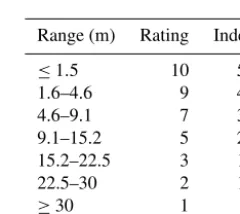
These data show that the depth varies from 1.50 m to more than 120 m. As in Dhundi et al. (2009), for depth beyond 100 m we assigned a rating of 0 because it is almost impossi-ble for pollutants to reach groundwater due to processes like sorption, filtration, biodegradation and volatilization. Table 1
Table 1.Range and rating for depth of water.
Range (m) Rating Index
≤1.5 10 50
1.6–4.6 9 45
4.6–9.1 7 35
9.1–15.2 5 25
15.2–22.5 3 15
22.5–30 2 10
≥30 1 5
Weight: 5
shows all the values for weight and scores for groundwater static level depth, and maps of the area are shown in Fig. 1.
To generate the map we used the inverse distance mov-ing average to get good accuracy (Samake et al., 2010, 2011). We assigned sensitivity rating values as in Dhundi et al. (2009): forD <1.5 m we assigned a rating ofr=10; if 1.5 m <D< 4.6 m then r=9; if 4.6 m <D< 9.1 m then
r=7; 9.1 m <D< 15.2 m then r=5; 15.2 m <D< 22.5 m thenr=3; if 22.5 m <D< 30 m thenr=2 and ifD> 30 m and the region has no data we assigned the rating valuer=1. 2.1.2 Recharge
disper-Table 2.Range and rating for net recharge.
Range (mm year−1) Rating Index
20–50 1 3
50–100 3 9
100–300 6 18
Weight: 3
Figure 2.Groundwater recharge distribution map.
sion, dilution, etc. will increase in unsaturated zones also. There are many sources of recharge in the study area, in-cluding precipitation, irrigation, waste water, return flow and infiltration from surface water (rivers, springs, etc.).
Net recharge data were taken from a report on the hydroge-ological synthesis of Mali (Mali Groundwater Resource In-vestigation, 1990). The different values of net recharge are in Table 2. Figure 2 represents the recharge map.
We used the following formula to calculate net recharge: net recharge=(rainfall−evaporation)×recharge rate. 2.1.3 Aquifer media
Aquifer media has been previously defined by many re-searchers: it describes rocks (consolidated and unconsoli-dated) which are used as water storage (Chandrashekhar et al., 1999). According to Heath (1987) an aquifer is an under-ground rock or deposit unit that will produce enough water to a borehole. The aquifer is also designated as a geological or hydrogeological formation which can produce enough water for consumption (Anwar et al., 2003). It is very important for attenuating pollution because it is the media where all reac-tions take place, and grain size and sorting are very important
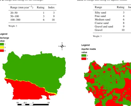
Table 3.Range and rating for aquifer media.
Range Rating Index
Silty sand 3 9
Fine sand 4 12
Medium sand 6 18
Coarse sand 8 24
Gravel and sand 9 27
Gravel 10 30
Weight: 3
Figure 3.Aquifer media distribution map.
in pollutant attenuation. Also the aquifer media governs flow path and length in an aquifer. Hence Piscopo (2001) indicates that the duration of time available for attenuation is deter-mined by the path length. In this study, we used topographi-cal map and well log data to prepare the aquifer media map. We assigned high rating values to coarse media and low val-ues to finer media. With the Mali hydrogeological synthesis maps and report on Senegal River basin groundwater simula-tions, the aquifer media data (Table 3) for this research were computed (Fig. 3) from more than 2300 boreholes.
2.1.4 Soil media
Table 4.Range and rating for soil media.
Range Rating Index
Gravel 10 20
Sand 9 18
Sandy loam 6 12
Loam 5 10
Silty loam 4 8
Clay loam 3 6
Weight: 2
Figure 4.Soil type distribution map.
The permeability of the soil media was used as a basis for assigning ratings on a scale of 1 to 10. The coarsest soils were assigned a rating of 10 and this decreased all the way to the finest media, which were assigned a rating of 1. Details of rating and index are shown on Table 4, while the soil map is shown in Fig. 4.
2.1.5 Topography
Topography of an area accounts for the change in slope. It is a determining factor of how rainfall and pollutants will ei-ther overflow or infiltrate (Lynch et al., 1994). The longer the water and/or pollutant is retained in an area, the greater the chance for infiltration is and, consequently, the higher the potential for recharge. Gentler slopes (slopes of 0–2 %) have higher retaining capacity for water and/or pollutants while steeper slopes (slopes of+18 %) have lower retention capacity for water and/or pollutants. According to Aller et
Table 5.Range and rating for topography (slope).
Range (%) Rating Index
0–2 10 10
2–4 9 9
10–12 5 5
14–16 3 3
Weight: 1 (Ckakraborty, 2007)
Figure 5.Slope distribution map.
al. (1987), topography has an effect on attenuation since it influences soil development.
Slope values extracted from a DEM of the region were reclassified and ranked on a scale (Table 5) of 1 to 10 to build the topography map (Fig. 5). This served as the basis of the multi-criteria analysis, in which other DRASTIC factors play a role.
2.1.6 Impact of vadose zone
The unsaturated or vadose zone is situated between the ground surface and groundwater table. It greatly impacts aquifer pollution potential due to its permeability, reactions, etc. (Corwin et al., 1997). Because the vadose zone is closely related to soil media and groundwater depth, we used the for-mula developed by Piscopo (2001) to estimate
Ir=Dr+Sr, (3)
whereIis the impact of vadose zone,Dis water table depth,
Table 6.Range and rating for vadose zone.
Range Rating Index
Clay and silt 3 15
Sandy clay 4 20
5 25
Clay sand 6 30
7 35
Sand and gravel 8 40
9 45
10 50
Weight: 5
Figure 6.Vadose zone distribution map.
For groundwater depth we chose the following ratings: 5 for depths less than 10 m, 2 for zones with depths between 10 and 30 m and 1 for regions where the water table static level is higher than 30 m. Similarly we chose 5, 3 and 1 for, respectively, high-, medium- and low-permeability soils. Fi-nally, we combined the two map layers to get the impact of vadose zone layer (Table 6 and Fig. 6).
2.1.7 Hydraulic conductivity
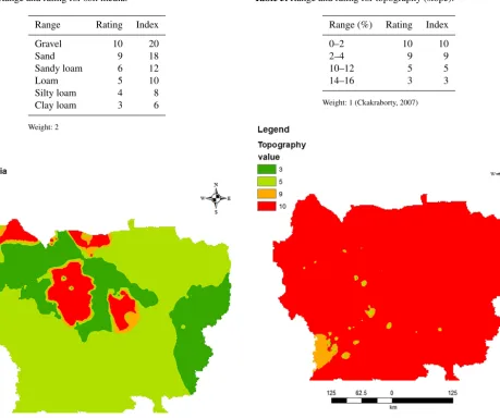
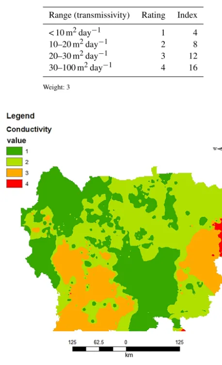
Hydraulic conductivity is the aquifer’s capacity to transport contaminants (Ckakraborty, 2007). It plays a very important role in aquifer contamination potential because an aquifer with a high value of C is more easily contaminated and one with a low value of C is not (Fritch et al., 2000).
Table 7.Range and rating for hydraulic conductivity.
Range (transmissivity) Rating Index
< 10 m2day−1 1 4
10–20 m2day−1 2 8
20–30 m2day−1 3 12
30–100 m2day−1 4 16
Weight: 3
Figure 7.Hydraulic conductivity distribution map.
We used transmissivity values instead of hydraulic con-ductivity to build the map. We adopted the following rating system: for very high values (> 450 m2day−1) we chose 10; for high values (300–450 m2day−1) we chose 8; for mod-erate values (100–300 m2day−1) we assigned 6; for moder-ately low values (30–100 m2day−1) we assigned 4; for low values (20–30 m2day−1) we chose 3; for very low values (10–20 m2day−1) we chose 2; and for extremely low values (< 10 m2day−1) we assigned 1 as the rating value. The dif-ferent values and distribution of hydraulic conductivity are shown in Table 7 and Fig. 7.
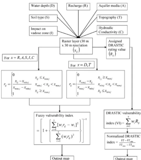
ta-Figure 8. Flow chart of methodology adopted to develop the groundwater contamination potential map using DRASTIC and fuzzy pattern recognition models in the framework of GIS (source Pathak et al., 2009).
ble is shallow, the recharge rate is high, and if aquifer and soil materials are coarser, groundwater potential for pollution is higher. Also if the hydraulic conductivity, recharge rate and slope are low then the groundwater potential for pollution is low. The main concept using fuzzy logic is very simple: it expresses whether a statement is true or untrue as well as the degree of verity or wrongness for all the inputs (Pathak et al., 2009). A function of membership links all fuzzy sets. We coupled fuzzy optimized model with GIS to evaluate the vul-nerability degree by converting the study area into a raster map and taking into account membership degrees in contin-uous passage from the highest polluted points to the lowest polluted points in hydrogeological settings.
Optimized fuzzy model
The fuzzy nature of groundwater vulnerability and ground-water vulnerability assessment can be considered as a par-ticular property. For example, instead of numerical measure-ment of factors in the DRASTIC method, the fuzzy method describes continuously the links between those factors that affect groundwater.
The fuzziness can be expressed continuously by member-ship degrees from 0 to 1. The following optimized model is used (Pathak et al., 2009).
Given a factor matrix,
X=(xij)7·n, (4)
where xij denotes the value of tester j in element i
(i=1,. . . ,7;j=1,. . . ) and nis the overall number of sam-pling points.
We can classify DRASTIC factors into two main groups. – Group 1: the increasing of parameter value increases
groundwater vulnerability to pollution.
– Group 2: the increasing of parameter value decreases groundwater vulnerability to pollution.
This membership degree can be expressed mathematically for group 1 as
rij
0 if xij ≤xminj
xij−xminj
xmaxj−xminj
1 if xij ≥xmaxj
if xminj ≥xij ≥xmaxj , (5)
and for group 2 as
rij
0 if xij ≥xmaxj
xmaxj−xij
xmaxj−xminj
1 if xij ≤xminj
if xminj ≥xij ≥xmaxj , (6)
whererij is the degree of membership for the samplej in
factori, minj is the smallest value of elementi (i.e., 1) in
the DRASTIC method and maxj is the maximum value of
elementi(i.e., 10) in the DRASTIC method.
We can use Eqs. (4), (5) and (6) to get the following matrix for the connection of factors:
R= rij7n, (7)
with the following conditions for matrixR:
– ifrij=1 then the testerj has the highest potential for
groundwater pollution according elementionly; – ifrij=0 then the testerj has the lowest potential for
groundwater pollution according the elementionly. For example, when all element connection degrees to highest potential for groundwater pollution are 1, then
Rij=(1, . . .,1). (8)
When all element connection degrees to lowest potential for groundwater pollution are 0, then
Rij=(0, . . .,0). (9)
So the membership degree of each or the parameters in sam-plejis
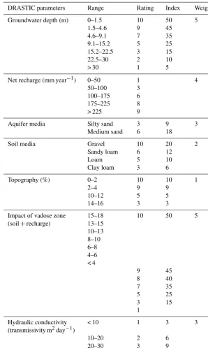
Table 8.DRASTIC parameters.
DRASTIC parameters Range Rating Index Weight
Groundwater depth (m) 0–1.5 10 50 5
1.5–4.6 9 45
4.6–9.1 7 35
9.1–15.2 5 25
15.2–22.5 3 15
22.5–30 2 10
> 30 1 5
Net recharge (mm year−1) 0–50 1 4
50–100 3
100–175 175–225 > 225
6 8 9
Aquifer media Silty sand 3 9 3
Medium sand 6 18
Soil media Gravel 10 20 2
Sandy loam 6 12
Loam 5 10
Clay loam 3 6
Topography (%) 0–2 10 10 1
2–4 9 9
10–12 14–16
5 3
5 3
Impact of vadose zone (soil+recharge)
15–18 13–15 10–13 8–10 6–8 4–6 < 4
10 50 5
9 45
8 7 5 3 1
40 35 25 15
Hydraulic conductivity (transmissivity m2day−1)
< 10 1 3 3
10–20 2 6
20–30 30–100
3 4
9 12
In the DRASTIC system different parameters have different weights (from 5 to 1) in relation to vulnerability; these are normalized in the evaluation process to sum to 1.
Let the weight vector be
W =(w1, . . ., w7)T . (11) The distance from one given samplej to the sample with the highest potential for groundwater pollution can be expressed as
d1= p v u u t
7 X
i=1
wi rij−1 p
. (12)
d2= p v u u t 7 X
i=1
(wirij)p. (13)
pin Eqs. (11) and (12) is the distance factor; whenp=1 the distances are called Hamming distances and whenp=2 the distances are called Euclidean distances.
We used Euclidean distances in our study. We can see clearly that ifd1=0 then the given samplej has the high-est potential for groundwater pollution and whend2=0 then the given samplej has the lowest potential for groundwater pollution.
Let the membership degree of the highest potential for groundwater pollution be denoted byujfor a given samplej,
so the membership degree of the lowest potential for ground-water pollution will be (1−uj) for the same given sample.
Membership can be regarded as weight in the fuzzy con-cept. So the following equations express more clearly contin-uous changes from a given samplej to the highest potential for groundwater pollution as well as from the same given sample to the lowest potential for groundwater pollution.D1 is the weighted distance to the highest potential for ground-water pollution.
D1=uj p v u u t 7 X i=1
wi rij−1 p
(14)
D2 is the weighted distance to the lowest potential for groundwater pollution.
D2=(uj−1)p v u u t 7 X
i=1
(wirij)p (15)
To get an optimized solution foruj the objective function
must be
minnF uj
=D12+D22o=u2j
( 7 X
i=1
wi rij−1 p
)2/p
+(1−uj)2 ( 7
X i=1
wirijp )2p
. (16)
After differentiating and solving Eq. (14), it becomes
uj= 1+ 7 P i=1 h
wi(r
ij−1) ip
7 P i=1
wirij p
2/p
. (17)
Equation (16) is called the fuzzy optimization model; the higher the value ofuj, the higher the potential for
groundwa-ter vulnerability to pollution for a given tesgroundwa-terj. This model
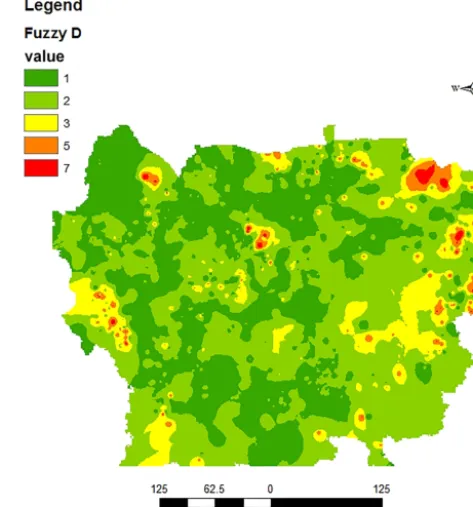
Figure 9.Fuzzy concept groundwater depth distribution map.
is joined to GIS and used to evaluate the pollution potential of groundwater. The diagram of procedures used to evaluate the map using DRASTIC and fuzzy methods in GIS is shown in Fig. 8.
3 Results and discussion
3.1 Fuzzy and DRASTIC parameters
Using memberships defined by fuzzy concept, groundwater table depth and topography maps were different from those of DRASTIC, but for the other five parameters the fuzzy op-timized and DRASTIC maps were identical.
The groundwater table depth and topographic maps ob-tained by using fuzziness are shown in Fig. 9 and 10. 3.2 Aquifer vulnerability maps
Figure 10.Fuzzy concept topography (or slope) distribution map.
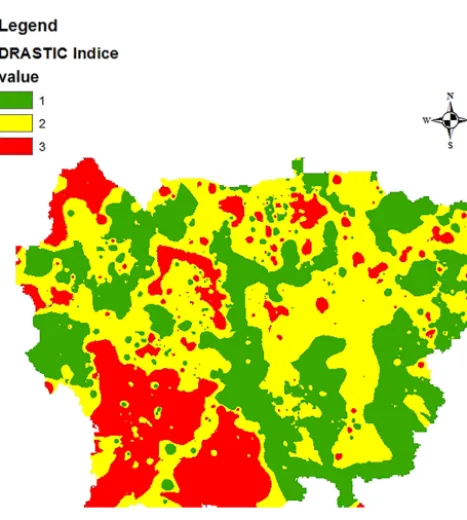
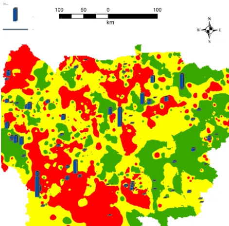
Figure 11.DRASTIC vulnerability map.
These values range from 72 to 141 and are classified into three distinct classes.
To facilitate and control scientific discussion, we used nat-ural break (jenks) classification to get three vulnerability
Figure 12.Normalized vulnerability map.
maps for both methods: the normalized DRASTIC method and fuzzy DRASTIC method.
Under these conditions Fig. 11 (DRASTIC method) shows that high-risk areas of Senegal basin in Mali are mainly sit-uated in the northern and southwestern portion of the basin with 14.64 % of total Senegal basin in Mali. The moderate risk areas, which cover 6.51 % of the total basin, are some-what disseminated and are mostly situated in the central and northern portion of the basin. Certain moderate risk areas are seen in the northeastern and western zones. All other portions of the Senegal basin in Mali are at low risk (78.85 %) and are found in the western and midwestern regions of the basin.
For the normalized vulnerability we found 21.68 % for high vulnerability, 15.22 % for moderate vulnerability and 63.32 % for low vulnerability. The map is shown in Fig. 12.
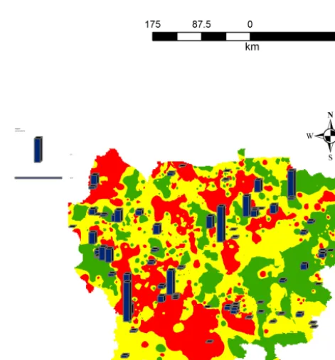
For the fuzzy DRASTIC method we found 18.92 % for the high-vulnerability zone, 8.94 % for the moderate-vulnerability zone and 72.11 % for the low-moderate-vulnerability zone (Fig. 13).
Table 9.Statistical summary of the seven parameters for the two methods.
D R A S T I C
d f d f d f d f d f d f d f
Min 1 0.33 1 0 3 0.22 3 0.22 3 0 3 0.22 1 0
Mean 5.52 0.5 1.36 0.04 4.27 0.36 5.71 0.52 9.83 0.02 8.14 0.79 1.93 0.10
Max 7 1 3 0.22 6 0.55 10 1 10 0.77 10 1 4 0.33
SD 1.41 0.16 0.77 0.08 1.48 0.16 2.20 0.24 0.72 0.08 1.24 0.13 0.87 0.09
Noted: d indicates the DRASTIC method and f is the fuzzy method.
Figure 13.Fuzzy DRASTIC vulnerability map.
of the study had different vulnerability indexes according to each method.
However, Figs. 14–16 show that the coincidence ratio with high nitrate concentration for the fuzzy DRASTIC method is the highest (81.13 %), followed by the normal-ized DRASTIC method (79.54 %) and finally the DRAS-TIC method (77.31 %). This confirmed our assertion that the fuzzy method better assesses groundwater vulnerability to pollution than the simple DRASTIC method.
3.3 Sensitivity analysis
Seven hydrogeological parameters influence the transport of the contaminants to aquifers when using the DRASTIC ap-proach. According to Rosen (1994), the high number of pa-rameters is intended to decrease indecision associated with using the individual parameters on the results. However, sev-eral researchers (Merchant, 1994; Barber et al., 1994) opine
Figure 14.Nitrate distribution in the DRASTIC model.
that groundwater risk assessment is possible without using all seven parameters of the DRASTIC method. Other re-searchers (Napolitano and Fabbri, 1996) also criticized that the weights and the ratings for the seven parameters are as-sumed for DPI assessment and lead to uncertainties about the precision of the outcomes for pollution risk assessment. Many factors contribute to the output of the DRASTIC model (Rahman, 2008; Ckakraborty, 2007) including map units in each layer, the weights, the overlay operation type that is per-formed, the number of data layers, the error or doubt associ-ated with each map unit, etc.
Sensitivity analysis was adopted to complement trial ev-idence for the DRASTIC method to perfect the uncertainty about model precision.
Two sensitivity analyses were then completed (Babiker et al., 2005; Lodwick et al., 1990): the map removal sensitivity test and the single parameter sensitivity analysis.
Figure 15.Nitrate distribution in the normalized model.
Figure 16.Nitrate distribution in the fuzzy model.
layer map and is applied using the following:
S=
V
N−
V0 N
V
·100. (18)
Sis the sensitivity degree,V is the unperturbed risk index us-ingNdata layers andV0is the perturbed risk index withN0
data layers. The real indexV is found by using all seven
pa-Table 10.Map removal sensitivity analysis (one parameter is re-moved at time).
Parameters removed Variation index (%)
Max Mean Min SD
D 3.69 1.72 0 0.76
R 2.99 1.58 0 0.44
A 3.61 0.67 0 0.42
S 2.99 0.83 0 0.42
T 3.40 0.92 0.06 0.18
I 7.19 3.60 0 0.88
C 4.85 1.53 0.05 0.38
Table 11.Map removal sensitivity analysis (one or more parameters are removed at time).
Parameters removed Variation index (%)
Max Mean Min SD
DASTIC 2.99 1.58 0 0.44
DASTI 5.71 3.73 1.38 0.72
DASI 8.44 6.06 2.92 0.88
DAI 13.18 9.49 4.32 1.54
DI 22.04 15.76 1.94 2.72
I 43.18 21.63 0 5.33
rameters whileV0can have a smaller number of parameters for the calculation procedure.
To estimate the impact of individual parameter on the risk potential, we used the single parameter sensitivity test. Dur-ing this test we compared the effective or actual weight of ev-ery individual factor with its hypothetical or allocated weight by using the following:
W=Pr·Pw
V ·100. (19)
W is the actual weight of the factor,Pr is the rating,Pw is
the weight andV is the risk index.
The statistical summary of all parameters is shown in Ta-bles 8 and 9. We noted that by using the DRASTIC method and Eq. (17) the highest vulnerability source is topography, which has a mean value of 9.83. The second main parame-ter affecting the risk is the impact of the vadose zone (8.14), followed by soil media (5.71). After the vadose zone comes groundwater table depth, with a mean value of 5.52. The fifth and the sixth positions are occupied, respectively, by aquifer media (4.27) and hydraulic conductivity (1.93) for their contribution to groundwater pollution potential. Finally net recharge showed the least mean value for contribution to pollution risk in Senegal basin in Mali.
Table 12.Single parameter sensitivity analysis (effective weights).
Parameters Theoretical Theoretical Effective weight (%) SD weight weight (%) Max Mean Min
D 5 21.73(22) 43.20 24.17 4.42 5.59
R 4 17.39(17) 15.58 4.80 2.85 2.65
A 3 13.04(13) 23.37 11.25 6.71 3.65
S 2 8.69(9) 21.97 10,04 4.61 3.70
T 1 4.34(4) 13.88 8.73 2.41 1.09
I 5 21.73(22) 57.47 35.92 14.27 5.37
C 3 13.04(13) 13.95 5.09 2.14 2.27
24.17 %. They are followed by aquifer media (11.25 %), soil media (10.04 %) and topography (8.73 %). Hydraulic con-ductivity and net recharge have relatively low variations with, respectively, 5.09 and 4.80 %. A low percentage means a small influence on variation of DPI across the basin.
Table 8 shows statistics and the correlation of the seven parameters used in both the DRASTIC and the fuzzy model. The average values of factors show that the vadose zone con-tributes the most DPI, with a mean value of 35.90 % for the DRASTIC and 0.79 for fuzzy membership. Depth of the wa-ter table (24.17 % and 0.5), aquifer media (11.24 % and 0.36) and soil media (10.02 % and 0.52) have a moderate contribu-tion to the final vulnerability index. Topography (8.72 % and 0.02), hydraulic conductivity (5.08 % and 0.1) and recharge (4.8 % and 0.04) have a low contribution to the final vulner-ability index.
3.4 Map removal sensitivity analysis
The first step of this test shows the change in DPI value when we remove only one map layer at a time. Tables 10 and 11 give the calculation results. Because the overall mean vari-ation is not more that 1 %, the test does not describe very clearly DPI variation when removing only one map layer at a time; also, all mean values are almost the same. However, the maximum value of DPI variation was estimated when we removed the unsaturated zone parameter map with a relative mean variation of 3.60 %. This can be explained by its rela-tively high theoretical weight in the DRASTIC method and the nature of unsaturated zone material in the basin. Moder-ate variations were seen after removal of groundwModer-ater table depth (1.72 %), net recharge (1.58 %) and hydraulic conduc-tivity (1.53 %). Only minor variations in mean values of DPI were noted (from 0.67 to 0.92 %) after removal of each of the other parameters from computation (Table 10).
The second step of the map removal sensitivity test shows the change in DPI value when we remove one or more map layers (or parameters) at a time from calculation. Based on the first step we removed parameters in the second step (Rah-man, 2008; Babiker et al., 2005) by preferentially removing the parameters, which produced less variation on the final DPI value and then the next smaller, and so forth.
The smallest mean effective weight variation was seen af-ter removal of net recharge (4.80 %) from the calculation. The more data layers we remove from calculation, the more the mean variation value increases because we keep the most effective parameters each time (Babiker et al., 2005). 3.5 Single parameter sensitivity analysis (effective
weight)
The significance of each of the seven parameters has been shown in map removal sensitivity analysis. Now we need to understand whether the theoretical weight affected by each parameter in the DRASTIC model is its actual/real or effec-tive weight after computation.
The actual weight represents the importance of the single factor compared with the other six factors and the weight given to it by the DRASTIC model (Rahman, 2008; Babiker et al., 2005). The single factor sensitivity test data can be seen in Table 12. The theoretical weight of both impact of unsaturated zone and groundwater static level is 21.73 % but their actual or effective weights are, respectively, 35.92 and 24.17 %. Because their actual weight is higher than their hy-pothetical (assigned) weight we can say that they are the two most effective factors (or parameters) in this DPI calculation. The soil media parameter (10.04 %) and topography parame-ter (8.73 %) similarly indicate large effective weight in com-parison to their theoretical weight (8.69 and 4.34 %, respec-tively). In contrast, the other three parameters presented less effective weight.
The importance of the four most effective parameters fo-cuses on the need for precise data for building the model. The low recharge and hydraulic conductivity values in the Senegal basin contribute to reducing the significance of these parameters in the groundwater vulnerability assessment.
4 Conclusion
Analyses were done with the purpose of observing the cor-relation between the intrinsic risk evaluation outcome and groundwater pollution in Senegal basin in Mali. DPI main values were low, moderate and high. In this study, a method-ology was adopted to improve DPI calculation to produce a pollution potential map. This was achieved by including the homogeneous nature of vulnerability to pollution using DRASTIC factors in a vast area. In addition, field measured nitrate data were used to confirm the risk of pollution of the Senegal basin. Thus, we can say that passing from ground-water that is easiest to pollute to most difficult to pollute can be continuous. This proves in fact the fuzzy nature of risk to groundwater pollution. So, a combined GIS-built fuzzy design model produces a continuous risk assessment func-tion, different levels of DRASTIC index, that is more accu-rate than the simple DRASTIC method. We compared simple DRASTIC, normalized DRASTIC and fuzzy DRASTIC out-puts and it appeared that fuzzy index coincides the most with nitrate distribution in the study area. The outputs show that 18.92 % of the study area’s groundwater aquifer is at a high risk of pollution due to fuzzy DRASTIC while 14.64 % of the study area’s groundwater aquifer is at a high risk of pollution from the simple DRASTIC method.
From this outcome, it can be established that risk de-termined by the fuzzy method is more consistent than the DRASTIC method. For several aspects of the local and re-gional groundwater resource protection and management, the maps of groundwater risk to pollution established in this work are important tools in policy- and decision-making.
Data availability. Data can be accessed by emailing the
corre-sponding author.
Competing interests. The authors declare that they have no conflict
of interest.
Acknowledgements. The authors would like to acknowledge
and thank the Government of Mali represented by the National Laboratory of Water (LNE), the National Directorate of Hydraulics, and the China University of Geosciences for their financial and technical support.
Edited by: Rosa Lasaponara
Reviewed by: Sidibe Aboubacar Modibo and one anonymous referee
References
Afshar, A. I., Marino, M. A., Asce, H. M., Ebtehaj, M., and Moosa V. J.: Rule based fuzzy system for assessing groundwater vulner-ability, J. Environ. Eng., 133, 532–540, 2007.
Alemi-Ardakani, M., Milani, A. S., Yannacopoulos, S., and Shok-ouhi, G.: On the effect of subjective, objective and combinative weighting in multiple criteria decision making: a case study on impact optimization of composites, Expert Syst. Appl., 46, 426– 438, 2016.
Aller, L., Truman, B., Rebecca, J. P., and Glen, H.: DRASTIC: a standardized system for evaluating groundwater pollution poten-tial using hydrogeologic settings, CR-810715, U.S. Geological Survey, Environmental Protection Agency, 1987.
Anoh, K.: Évaluation de la vulnérabilité spécifique aux intrants agri-coles des eaux souterraines de la région de Bonoua, Mémoire de DEA, Université de Cocody, Cocody, 68 pp., 2009.
Antonakos, A. K. and Lambrakis, N. L.: Development and testing of three hybrid methods for assessment of aquifer vulnerability to nitrates, based on the DRASTIC model, an example from NE Korinthia, Greece, J. Hydrol., 333, 288–304, 2007.
Anwar, P. and Rao, M.: Evaluation of groundwater potential of Musi River catchment using DRASTIC index model, in: Hydrol-ogy and watershed management, edited by: Venkateshwar, B. R., Ram, M. K., Sarala, C. S., and Raju, C., Proceedings of the inter-national conference, 18–20, B.S. Publishers, Hyderabad (2003), 399–409, 2002.
Atkinson, S.: An examination of groundwater pollution potential through GIS modeling, ASPRS/ACSM, 1994.
Babiker, I. S., Mohammed, M., Hiyama, T., and Kato, K.: A GIS-based DRATIC model for assessing aquifer vulnerability in Kakamigahara Heights, Gifu Prefecture, central Japan, Sci. Total Environ., 345, 127–140, 2005.
Barber, C., Bates, L. E., Barron, R., and Allison, H.: Comparison of standardized and Region-specific methods assessment of the vulnerability of Groundwater to pollution: A case study in an Agricultural catchment, in: Proceedings of 25th IAH Congress water Down under, Melbourne, Australia, 1994.
Bezelgues, S., Des, G. E., Mardhel, V., and Dörfliger, N.: Car-tographie de la vulnérabilité de Grand-Terre et de Marie-Galatie (Guadeloupe). Phase 1: Méthodologie de détermination de la Vulnérabilité, 2002.
Bojórquez-Tapia, L. A., Cruz-Bello, G. M., Luna-González, L., Juárez, L., and Ortiz-Pérez, M. A.: V-DRASTIC: using visual-ization to engage policymakers in groundwater vulnerability as-sessment, J. Hydrol., 373, 242–255, 2009.
Chandrashekhar, H., Adiga, S., Lakshminarayana, V., Jagdeesha, C. J., and Nataraju, C.: A case study using the model “DRASTIC” for assessment of groundwater pollution potential, in: Proceed-ings of the ISRS national symposium on remote sensing applica-tions for natural resources, June 1999, 19–21, Bagalore, 1999. Civita, M.: La Carte Della Vulnerabilità Degli Acquiferi
All’inquiamento: Teoria e Pratica, edited by: PITAGORA, Bologna, 1994.
Corwin, D. L., Vaughan, P. J., and Loague, K.: Modeling non-point source pollutants in the vadose zone with GIS, Envir. Sci. Tech., 31, 2157–2175, 1997.
Denny, S. C., Allen, D. M., and Journea, Y. J.: DRASTIC-Fm: a modified vulnerability mapping method for structurally con-trolled aquifers in the southern Gulf lslands, British Columbia, Canada, Hydrogeol. J., 15, 483–493, 2007.
Dhar, A.: Geostatistics-based design of regional groundwater mon-itoring framework, ISH J. Hydraul. Eng., 19, 80–87, 2013. Dhar, A. and Patil, R. S.: Multiobjective design of groundwater
monitoring network under epistemic uncertainty, Water Resour. Manage., 26, 1809–1825, 2012.
Dhar, A., Sahoo, S., Dey, S., and Sahoo, M.: Evaluation of recharge and groundwater dynamics of a shallow alluvial aquifer in Cen-tral Ganga Basin, Kanpur (India), Nat. Resour. Res., 23, 409– 422, 2014.
Dhundi, R. P., Akira, H., Isao, A., and Luonan, C.: Groundwater vulnerability assessment in shallow aquifer of Kathmandu Val-ley using GIS-based DRASTIC model, Environmental Geology, 1569–1578, 2009.
Engel, B., Navulur, K., Cooper, B. S., and Hahn, L.: Estimating groundwater vulnerability to non point source pollution from ni-trates and pesticides on a regional scale, Int. Assoc. Hydrol. Sci. Publi., 235, 521–526, 1996.
Fernando, A. L. P. and Luís, F. S. F.: The multivariate statistical structure of DRASTIC model, J. Hydrol., 476, 442–459, 2013. Fritch, T. G., McKnight, C. L., Yelderman Jr., J. C., and Arnold,
J. G.: An aquifer vulnerability assessment of the paluxy aquifer, central Texas, USA, using GIS and a modified DRASTIC ap-proach, Environ. Manage., 25, 337–345, 2000.
Hamza, M. H.: A GIS-based DRASTIC vulnerability and net recharge reassessment in an aquifer of a semi-arid region Metline-Ras Jebel-Raf Raf aquifer, Northern Tunisia, 2006. Hamza, M. H., Added, A., Frances, A., and Rodriguez, R.: Validité
de l’application des méthodes de vulnérabilité DRASTIC, SIN-TACS et SI à l’étude de la pollution par les nitrates dans la nappe phréatique de Metline-Ras Jebel-Raf Raf (Nord-Est Tunisien), Geoscience, 339, 493–505, 2007.
Hearne, G.: Vulnerability of the uppermost groundwater to contam-ination in the greater Denver Area, Colorado, USGS water re-sources investigation report 92-4143, 241 pp., 1992.
Heath, R. C.: Basic Groundwater Hydrology, US Geological Survey Water Supply paper 2220, US Department of the Interior, US Geological Survey, 1987.
Jha, M. K.: Vulnerability Study Of Pollution Upon Shallow Ground-water Using Drastic/GIS, 2005.
Jourda, J. P., Saley, M. B., Djagoua, E. V., Kouame, K. J., Biemi, J., and Razack, M.: Utilisation des données ETM+de Landsat et d’un SIG pour l’évaluation du potentiel en eau souterraine dans le milieu fissure précambrien de la région de Korhogo (nord de la Côte d’Ivoire): approche par analyse multicritère et test de vali-dation. Revue de Télédetection, 5, 339–357, 2006.
Jourda, J. P., Kouame, K. J., Adja, M. G., Deh, S. K., Anani, A. T., Effini, A. T., and Biemi, J.: Evaluation du degré de pro-tection des eaux souterraines: vulnérabilité à la pollution de la nappe de Bonoua (Sud-Est de la Côte d’Ivoire) par la method DRASTIC, Actes de la Conférence Francophone, SIG 2007/ 10 au 11 Octobre 2007, Versailles-France, 11 pp., available at: www.esrifrance.fr/SIG2007/Cocody_Jourda.htm, 2007.
Kalinski, R.: Correlation between DRASTIC vulnerabilities and in-cidents of VOC contamination of municipal wells in Nebraska, Groundwater, 32, 31–34, 1994.
Kouame, K. J.: Contribution à la Gestion Intégrée des Ressources en Eaux (GIRE) du District d’Abidjan (Sud de la Côte d’Ivoire): Outils d’aide à la décision pour la prévention et la protection des eaux souterraines contre la pollution, Thèse de Doctorat, Univer-sité de Cocody, Cocody, 250 pp., 2007.
Leone, A., Ripa, M. N., Uricchio, V., Deak, J., and Vargay, Z.: Vulnerability and risk evaluation of agricultural nitrogen pollu-tion for Hungary’s main aquifer using DRASTIC and GLEAMS models, J. Environ. Manage., 90, 2969–2978, 2009.
Lodwik, W. A., Monson, W., and Svoboda, L.: Attribute error and sensitivity analysis of maps operation in geographical informa-tion systems–suitability analysis, Int. J. Geograph. Inf. Syst., 4, 413–428, 1990.
Luis, A. B. T., Gustavo, M. C. B., Laura, L. G., Lourdes, J., and Mario, A. O. P.: V-DRASTIC: Using visualization to engage pol-icymakers in groundwater vulnerability assessment, J. Hydrol., 373, 242–255, 2009.
Lynch, S. D., Reynders, A. G., and Schulze, R. E.: Preparing input data for a national-scale groundwater vulnerability map of south-ern Africa, Document ESRI 94, 1994.
Madhumita, S., Satiprasad, S., Anirban, D., and Biswajeet, P.: Effectiveness evaluation of objective and subjective weighting methods for aquifer vulnerability assessment in urban context, J. Hydrol., 541, 1303–1315, 2016.
Merchant, J. W.: GIS-based groundwater Pollution hazard assess-ment a critical review of the DRASTIC model, Photogramm. Eng. Rem. S., 60, 1117–1127, 1994.
Mohamed, R. M.: Evaluation et cartographie de la vulnérabilité à la pollution de l’aquifère alluvionnaire de la plaine d’El Mad-her, Nord-Est algérien, selon la méthode DRASTIC, Sciences et changement planétaires, Sécheresse, 12, 95–101, 2001. Murat, V., Paradis, D., Savard, M. M., Nastev, M., Bourque, E.,
Hamel, A., Lefebvre, R., and Martel, R.: Vulnérabilité à la nappe des aquifères fracturés du sud-ouest du Québec: Evaluation par les methods DRASTIC et GOD, Ressources Naturelles Canada, Commission Géologique, 2003.
Napolitano, P. and Fabbri, A. G.: Single parameter sensitivity anal-ysis for aquifer vulnerability assessment using DRASTIC and SINTACS, in: Proceedings of the 2nd HydroGIS conference, IAHS Publication, Wallingford, 235, 559–566, 1996.
Neshat, A. and Pradhan, B.: An integrated DRASTIC model using frequency ratio and two new hybrid methods for groundwater vulnerability assessment, Nat. Hazards, 76, 543–563, 2015a. Neshat, A. and Pradhan, B.: Risk assessment of groundwater
pol-lution with a new methodological framework: application of Dempster-Shafer theory and GIS, Nat. Hazards, 78, 1565–1585, 2015b.
Newton, J. T.: Case study of Transboundary Dispute Resolution: Organization for the Development of the Senegal River (OMVS), Transboundary Freshwater Dispute Database, Oregon State Uni-versity, available at: http://www.transboundarywaters.orst.edu/ research/case_studies/OMVS_New.htm (last access: 26 Febru-ary 2012), 2007.
mapping using GIS, modeling and a fuzzy logic tool, J. Contam. Hydrol., 94, 277–292, 2007.
O.M.V.S.: Le Journal N.8 Octobre, available at: http://www. portail-omvs.org/actualite/omvs-journal-ndeg-8-octobre, 2013. Osborn, N. I., Eckenstein, E., and Koon, K. Q.: Vulnerability
as-sessment of twelve major aquifer in Oklahoma. Oklahoma Water Resources Boards, Technical Report, 1998.
Pacheco, F. A. L. and Van der Weijden, C. H.: Delimitation of recharge areas in the Sordo river basin using oxygen isotopes, in: VIII Congresso Ibérico de Geoquímica – XVII Semana de Geoquímica. Escola Superior Agrária do Instituto Politécnico de Castelo Branco, Castelo Branco, 6 pp., 2011.
Pacheco, F. A. L. and Van der Weijden, C. H.: Integrating topogra-phy, hydrology and rock structure in weathering rate models of spring watersheds J. Hydrol., 428–429, 32–50, 2012.
Pacheco, F. A. L., Pires, L. M. G. R., Santos, R. M. B., and Fernan-des, L. F. S.: Factor weighting in DRASTIC modeling, Sci. Total Environ., 505, 474–486, 2015.
Pathak, D. R., Hiratsuka, A., Awata, I., and Chen, L.: Groundwater vulnerability assessment in shallow aquifer of Kathmandu Valley using GIS based DRASTIC model, Environ. Geol., 57, 1569– 1578, https://doi.org/10.1007/s00254-008-1432-8, 2009. Piscopo, G.: Groundwater Vulnerability Map Explanatory Notes –
Castlereagh Catchment, Parramatta NSW, Australia NSW De-partment of Land and Water Conservation, 2001.
Rahman, A.: A GIS based DRASTIC model for assessing ground-water vulnerability in shallow aquifer in Aligarh, India, Appl. Geogr., 28, 32–53, 2008.
Rosen, L.: Study of the DRASTIC methodology with the emphasis on Swedish conditions, 37th conference of the International As-sociation for Great Lakes Research and Estuaire Research Fed-eration, Buffalo, p. 166, 1994.
Sahoo, S., Dhar, A., Kar, A., and Chakraborty, D.: Index-based groundwater vulnerability mapping using quantitative parame-ters, Environ. Earth Sci., 75, 1–13, 2016a.
Sahoo, S., Dhar, A., and Kar, A.: Environmental vulnerability as-sessment using grey analytic hierarchy process based model, En-viron. Impact Assess. Rev., 56, 145–154, 2016b.
Saidi, S., Bouria, S., Dhiaa, H. B., and Anselmeb, B.: Assessment of groundwater risk using intrinsic vulnerability and hazard map-ping: application to Souassi aquifer, Tunisian Sahel, Agric. Water Manage., 98, 1671–1682, 2011.
Samake, M., Zhonghua, T., Win, H., Innocent, M., and Kanya-manda, K.: Assessment of Groundwater Pollution Potential of the Datong Basin, Northern China, Journal of Sustainable De-velopment, 3, 140–152, 2010.
Samake, M., Zhonghua, T., Win, H., Innocent, M., Kanyamanda, K., and Waheed, O. B.: Groundwater Vulnerability Assessment in Shallow Aquifer in Linfen Basin, Shanxi Province, China Using DRASTIC Model, Journal of Sustainable Development, 4, 53– 71, 2011.
Sener, E., Sener, S., and Davraz, A.: Assessment of groundwater vulnerability based on a modified DRASTIC model, GIS and an analytic hierarchy process (AHP) method: the case of Egirdir Lake basin (Isparta, Turkey), Hydrogeol. J., 21, 701–714, 2013. Sinha, M. K., Verma, M. K., Ahmad, I., Baier, K., Jha, R., and
Az-zam, R.: Assessment of groundwater vulnerability using modi-fied DRASTIC model in Kharun Basin, Chhattisgarh, India, Ara-bian Journal of Geosciences, 9, 98–103, 2016.
Shirazi, S. M., Imran, H. M., Akib, S., Zulki, Y., and Harun, Z. B.: Groundwater vulnerability assessment in the Melaka State of Malaysia using DRASTIC and GIS techniques, Environmental Earth Sciences, 9, 1–22, 2013.
UNESCO: World Heritage related Category, available at: http:// whc.unesco.org/en/news/874, 2012.