A Predicate Based Fault Localization Technique Based On Test Case Reduction

380

_____________________

 Rohit Mishra Department of Computer Science & Information Technology,S.H.I.A.T.S, Nainy Allahabad Uttar Pradesh India 211007

 Dr. Raghav Yadav Department of Computer Science & Information Technology, S.H.I.A.T.S, Nainy Allahabad

Uttar Pradesh India 211007. E-mail:

[email protected], E-mail:

[email protected]

A Predicate Based Fault Localization Technique

Based On Test Case Reduction

Rohit Mishra, Dr.Raghav Yadav

ABSTRACT: In today‟s world, software testing with statistical fault localization technique is one of most tedious, expensive and time consuming acti vity. In faulty program, a program element contrast dynamic spectra that estimate location of fault. There may have negative impact from coincidental correctness with these technique because in non failed run the fault can also be triggered out and if so, disturb the assessment of fault location. Now eliminating of confounding rules on the recognizing the accuracy. In this paper coincidental correctness which is an effective interface is the reason of success of fault location. We can find out fault predicates by distribution overlapping of dynamic spectrum in failed runs and non failed runs and slacken the area by referencing the inter class distances of spectra to clamp the less suspicious candidate. After that we apply cov erage matrix base reduction approach to reduce the test cases of that program and locate the fault in that program. Finally, empirical result shows that our technique outshine with previous existing predicate based fault localization technique with test case reduction.

Keywords: Fault Localization, Predicates, Dynamic Spectrum, Coincidental correctness, Class distribution, Coverage base matrix

1

I

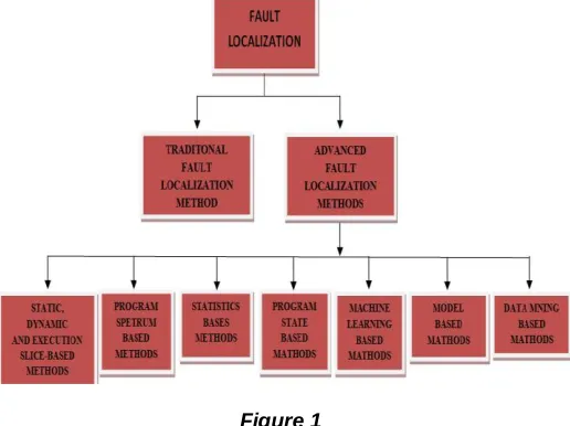
TODAY‟S software and system of software are going to be more complicated. The quality of software is becoming more important and effective mechanism for academia and industries. The failed program is the reason for fault existing in a program. Now to overcome from this, the programmer fixes a program fault and locates it first. There are several fault localization technique exist.

Figure 1

Although the statistic fault localization (SFL) technique is

Figure 2

outshine some representative existing predicate based SFL technique. Our paper is mannered as follows: In first section we propose a technique that estimates fault localization with the presence of coincidental correctness. It is requisite to be more accurate since there is no longer a need to discriminate the coincidental correctness runs.In second section of this paper we present our motivation and research aim.Section third elaborates our model to the related work. Section four gives the experimental evolution andmeasurement of the paper.Section five gives the related work.And finally we conclude our paper on section six.

2

2.1 THE SAMPLE PROGRAM

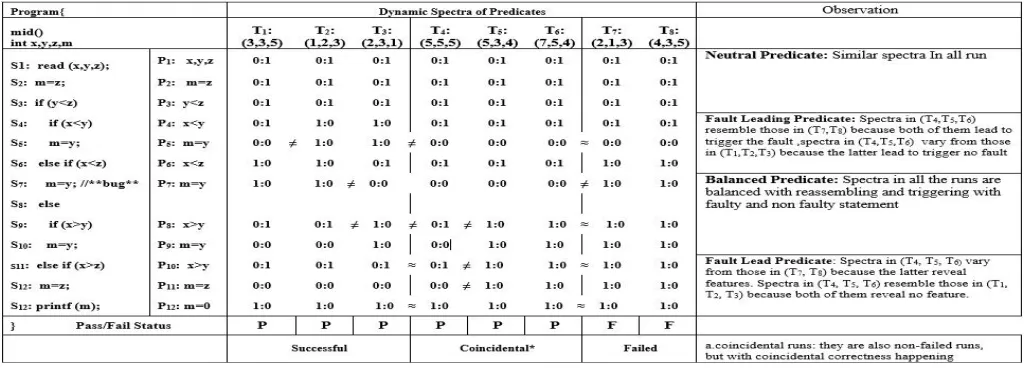
There is the example in Figure 2 shows a piece of code to find out the mid value among three inputs. A fault is seeds in the statement S7 which may be a reason of the program to

generate an incorrect output. We take three integer as an input to begin the program and permute them to create eight test cases named as; T1, T2, T3, T4 ,T5,T6, T7, T8. We notices that

the test cases from T4, T5and T6exercised the faulty statement

but only T7 and T8 give unexpected output. Thus we noted

down test case T7 and T8 as failed runs and other execution as

non fails runs. To make our discussion easier we introduce the word coincidental run, to name the program execution over T4,

T5 and T6where the fault is figured but no state is figured as

faulty observable. To differentiate from them we introduce the term successful runs to name the program runs over T1, T2and

T3. Now we are going to install 12 predicate in the program

named as P1, P2, P3, P4, P5, P6, P7, P8, P9, P10, P11, P12 in

above Figure 2. We also consider their dynamic spectrum in the form of x:y in the program which indicate the number of times the predicate is evaluated as true and evaluated as false respectively. Let us take first row to illustrate. In the test case of T1 predicate “P1: x=a” is evaluated false (0) ones and never

evaluated true. Thus we calculate dynamic spectra of predicate p1 as “0:1”in that run

2.2

I

O

W

As there is no loop in the program and it is execute sequentially, we introduce four categories of predicates named as: Neutral, Fault leading, Fault led and Balanced predicate

Now the twelve predicate are partitioned into group in which P1, P2 and P3 is neutral predicate P4, P5 and P6 fault leading

predicate P7,P8and P9 is balanced predicate and P10, P11 and

P12 is fault led predicates. Here we notice that predicate P4

most fault relevant predicate is fault leading predicate with such classification. In neutral predicate its dynamic spectra in every run resemble each other. We can understood as that there are very less chances to make relationship with fault so that their behavior makes less difference in every runs either it is a failed runs or non failed runs. If we can take the predicate P1 in the test case T4 to illustrate predicate “P1: x= =a” lies on

the first statement and always evaluate false and its spectra in all the runs are equal. For a fault leading predicates there is a difference in its dynamic spectra in coincidental runs (the non failed in coincidental correctness happening) are identical to those in run but different from those in successful runs (the non failed without coincidental correctness happening). We use the symbol “≠” and “≈” in Figure 2 to make a better view. We can elaborate is as, the execution paths leading to a fault often concentrate into small clusters as reported in [6]. That‟s why this predicate may revealed the similar dynamic spectra in both coincidental runs and failed runs. Let us take predicate P4 and test case T4 to illustrate. Predicate “P4: x<y” give false

which skip the statement S5 to triggers the false the statement

S7. This is the only legal way that leads the fault and for

predicate p4 in test case T4, their dynamic spectra are same to

those in T7 and T8 and different from T1, T2 and T3. In fault led

predicate the dynamic spectra are identical for coincidental run to those in the successful run and different from failed runs. We can elaborate it as if the fault is exercised the faulty state may be coincidentally not propagate and the led program still behave as normal. That‟s why there is no difference can be observed in the dynamic spectra from the successful run and coincidental run for fault led predicate. Let us take predicate P9

and program run (test case) T4 to illustrate. During program

run T4 even with the faulty value of x, predicate “P9: x>y” give

the correct solution (i.e evaluate false). The fault is glossed over which leads the rest program except (from S13 to the end)

to execute normal. Now the result in predicate P9 in the Test

case T4, their dynamic spectra are same to T1 and T2 and

different from T7 and T8. In balanced predicate thedynamic

382

coincidentally not propagate and the program still behave as normal. That‟s why there is no difference can be observed in the dynamic spectra from the successful run and coincidental run for balanced predicate.Let us take predicate P8 and

program run (test case) T4 to illustrate. During program run T4

even with the faulty value of x, predicate “P8: x>y” give the

correct solution (i.e evaluate false). The fault is glossed over which leads the rest program except (from S13 to the end) to

execute normal. Now the result in predicate P10 in the Test case T4, their dynamic spectra are balanced to T1, T2, T3 and

T4 but different from T5, T6, T7 and T8. Now with the help of

overlapping of spectrum distribution in failed run and non failed run can be effective means to differentiate a fault leading predicate from the other. As we mentioned above that the dynamic spectra of predicate P4 in test case T4 are same to

those in T7 and T8 and different from T2 and T3. So we record

the overlapping 100 percent in T4, T5, T6, T7 and T8. The same

mechanism is observed with the predicate P9, the dynamic spectra in T7 and T8 are not met in T4, T5, and T6 and record

the overlapping 0 percent for it. Thus these caparison which shows the overlapping rule out the fault led predicate. How does our model work in such types of cases? We will detail it in our model in the next section.

3

OUR

MODEL

A PROBLEM SETTING

Let P be a faulty program with n predicate that are referred to as p1, p2, p3… . . pn . Program run R is divided in two sets N

and F where N={n1, n2, n3… . . ny} for the y non failed runs and

F={f1, f2, f3… . . fv} for v failed runs. As we can see in our Figure

2 N={T1,T2,T3,T4,T5,T6} and F={T7,T8}.

Now we introduce the two term as eT (pj, ri) and eF (pj, ri) to

measure the number of times a predicate pj is evaluated as

trueor false for the number of program runs ri respectively.

B PRELIMINARIES

Before starting to elaborate our model we first introduce some preliminaries. Following previous studies [11] we use x(pj, ri)

to show the evolution bias of predicate pj in a program run ri.

Here an evolution bias is the probabilities of a predicate being evaluated true in a program run. It is calculated as-

x 𝐩𝐣, 𝐫𝐢 =

𝐞_𝐓 (𝐩_𝐣,𝐫_𝐢) 𝐞𝐓 𝐩𝐣,𝐫𝐢 +𝐞𝐅 (𝐩𝐣,𝐫𝐢)

We also use the term x pj, fi and x pj, ni to express the

evaluation bias of predicate pj in both failed and non failed

runs respectively. Further to denote the vector of evolution bias for each predicate in ith failed run fi , we have

𝐗𝐢𝐅= [x 𝐩𝟏, 𝐫𝐢 , x 𝐩𝟐, 𝐫𝐢 ………. x 𝐩𝐧, 𝐫𝐢 ]

WhereX_iF denote the vector of evaluation bias in the ith non failed run fi . Similarly XiT is denoted the vector of evolution

bias in the ith non failed run ni. Now the overlapping of

spectrum distribution in both failed and non failed run consider the similarity between two types of run. According to the evaluation bias which exists in both of them. In this paper to measure the overlapping, we introduce Bhattacharya coefficient [2]. This function is used to measure the overlapping amount between two statistical sample and population. Let pj and yj be the predicate and evaluation bias

respectively and wF and wN denotes failed runs and non failed

runs respectively.Bhattacharya coefficient can be formulized as:

BC (P (𝐲𝐣 𝐰𝐅), (𝐲𝐣 𝐰𝐍) = 𝐲𝐣∈𝐃𝐣 (𝐏 (𝐲𝐣 𝐰𝐅)× (𝐲𝐣 𝐰𝐍)

Where Di is the domain of yj and P(yj wF) and P(yj wN) are

the coincidental probabilities of yj in the set of failed and non

failed runs respectively. The probability of yj exists in both of

the two kinds of runs which are P(yj wF)× P(yj wN) . The

measure is proved to be the upper bond of Bayes error which directly related to the overlapping of two model. We use σjF v

and σjN u in this paper to approximate P(yj wF) and P(yj wN)

respectively. Where

σjF vis the kind of appearance of yj in the set of failed runs.

σjN uis the kind of appearance of yj in the set of non failed

runs. Now take the predicate p1 in our Fig-2 as an example

and we can see that there exists only one variable y1= 0 .So

conditional probability are P(y1 wF) and P(y1 wN) are 1and

BC (P(y1 wF), (y1 wN) = 1

C OUR TECHNIQUE

Our technique consists of five steps.

1GATHERING DYNAMIC SPECTRA:

Gathering dynamic spectra for all predicate in every test case and predicators are inserted in three kinds of statement i.e Branch statement, Scalar pair and Return statement. To capture the dynamic spectra we use evaluation bias.

2 CALCULATING THE OVERLAPPING OF DYNAMIC SPECTRUM: In both neutral and fault leading predicate since their dynamic spectra for failed run and coincidental run are reassemble each other to great extent. So we use the spectrum distribution overlapping to differentiate them from fault led predicate. Bhattacharya distance [2] is used to calculate the spectrum distribution in case of failed and non failed run.(note: we cannot figure out the coincidental run from the non failed runs). Now we have given a predicate Pj to determine the overlapping of its spectrum distribution in failed run F and in non failed run N. The overlapping Oj of the spectrum

distribution in both failed and non failed runs can be explained in terms of Bhattacharya distance:

𝐎𝐣 = -ln [BC (P(𝐲𝐣 𝐰𝐅), (𝐲𝐣 𝐰𝐍) ]

Where BC (∙) is Bhattacharya coefficient.

If BC (P (yj wF), (yj wN) = 0 we set Oj is to be+∞ .

After this step we may record all the predicate in descending order by referencing their overlapping values. The top ranked predicate contains more fault leading predicate. However we also predict that after such a step the neutral predicate may mix with fault leading predicate as well as balanced predicate in the result.

3 CALCULATING THE INTER AND INTRA CLASS DISTANCE:

and fault led predicates in successful and failed runs which are different from each other to a great extant. That‟s why we adopt to estimate the inter class distance to differentiate them from neutral predicate. The inter class distance Bj for a

predicate Pj is calculated as:

𝐁𝐣= 𝐦𝐣𝐅− 𝐦𝐣𝐍

Where mjF and mjN denotes mean value of the evaluation bias

for Pj in the failed and non failed test case respectively and m_jF and mjNare calculated as :

𝐦𝐣𝐅 = 𝟏_𝐯 [𝐱(𝐯𝐢=𝟏 𝐩𝐣, 𝐟𝐢)] and 𝐦𝐣𝐍 = 𝟏_𝐮 [𝐱(𝐮𝐢=𝟏 𝐩𝐣, 𝐧𝐢)]

The inter class distance Bjmeasure the distance between the

evaluation bias of predicate Pjin the set of both failed and non failed run respectively. In the motivation, we have explained that the inter class distance of neutral predicate is less than fault leading predicate and thus we can differentiate a neutral predicate from fault leading predicate.However we also realize that the spectrum distribution for two predicate may have unequal width, directly comparing their inter class distance may not be scientific. For example the predicate that installed for the branch statement of the long lops may have very small evaluation bias value3. So the inter class distance calculate for it can be much smaller than the average. Now if we want to fairly compare the inter class distance between two predicates, we introduce intra class distance. To normalize them before comparison. The intra class distance Djfor the predicate Pjis

calculated as;

𝐃𝐣 = [𝐱( 𝐯

𝐢=𝟏 𝐩𝐣,𝐟𝐢)−𝐦𝐣𝐅]𝟐

𝐯 +

[𝐱( 𝐮

𝐢=𝟏 𝐩𝐣,𝐧𝐢)−𝐦𝐣𝐧]𝟐 𝐮 𝟐

Similarly explained asBj. Note: it is the mean of intra class

distance of Pjfor failed and non failed run. Now we can normalized the inter class distance Bjusing the intra class

distanceDjfor each predicate so that their distance can be

fairly compared to each other. The normalized inter class distance Ajfor pjis as follows:

𝐀𝐣 = 𝐁_𝐣 𝐃𝐣

When Dj=0 andBjis not 0 then Aj=∞.

When Dj=0 andBjis also 0then Aj=0.

This step decreases the rank of the neutral predicate without affecting the relative order of the fault leading predicate and fault led predicate.

4

G

:

In previous step, we differentiate neutral predicate with fault leading predicate with the help of normalized inter class distanceAj. Now by integrating the suspiciousness formula Sj

as:

Sj= 𝟐(𝐎𝐣 −𝐀𝐣)

Since with the great use of Ojwe can rule out the fault led

predicate and the use of Ajwe can suppress neutral predicates. We thus identify fault leading predicate and balanced predicate. At the same time since the normalized inter class distance for fault leading predicate is supposed to be comparable to that of fault led predicate is still reserved by

the adjustment of “-Aj”. The base number 2 is to assure that Sj>0. Now finally rearrange the predicates in descending order of their suspiciousness score Sj and generate the rank list of predicates.

5

C

M

B

R

(CMR)

5.1 EXECUTION PATH

The execution path of a program P to be a sequence of statements that executes in a program P = <p1, p2,…, pi,…>. The P executed by test case t is denoted as PATH(t).

5.2 COVERAGE VECTOR

The coverage vector (binary vector) of test case t is denoted as COVER(t), where COVER(t)=<s′1, s′2, s′3,…,s′n> (n is the number of statements of P). In the program the statements which are execute its value is „1‟ otherwise „0‟.

s′j=1,PATH(t) covered in jth

statement or 0, PATH(t) uncovered in jth statement

5.3 COVERAGE MATRIX

Given a target program P, which consists of statements s1, s2,

…sn Let T ={t1,t2,…,tm} be a test-suite for P, m be the number

of test cases for

P.COVER(T)=COVER(t1),COVER(t2)…COVER(tm)}.

5.4 WEEKLY IRRELEVANT STATEMENT

The statements which are execute in all the test cases are called weakly irrelevant statement because these statement are not give any idea of fault localization that‟s why we remove those statement and create new vector which is known asRCOV(t). Let T ={t1,t2,…,tm} be a test-suite for program P, sk

(1≤k≤n) be one of statements of P, COVER(T) be the statement coverage matrix of P. sk is a weekly relevant

statement of P for the test-suite T, if and only if for all pairs of i and j (1≤i≤m; 1≤j≤m; i≠j), COVER(ti–sk)==COVER(tj–sk). COVER(ti–sk) is the kth

element of COVER(ti). By comparing the statistical difference in passed and failed test cases we can measure the dubious score of each statement. Weekly irrelevant statement is executed by all the passed and failed test cases, so the dubious score of weakly relevant statements are relative small. The remaining coverage matrix which does not contain the weakly relevant statements is denoted as RCOV(T), the remaining coverage vector corresponding to test cases ti is denoted as RCOV(ti), and the remaining coverage vector corresponding to fault-localization requirements FLreq is denoted as RCOV(FLreq).

384 5.5 FAULT LOCALIZATION REQUIREMENT VECTOR (FLREQ)

The FLreq is obtained by analyzing the coverage vectors of all failed test cases. Let T={t1,t2,…tm}be a failed test-suite for P.

The faulty statement should be executed by every failed test case for the localization of a single fault, so the statement executed by all the failed test cases should be included. FLreq = COVER(t1) ∩ COVER(t2) ∩… ∩ COVER(tm). By contrast, for

the localization of multiple faults, the program should contain several faulty statements. One failed test case may not execute all of the faulty statements but one faulty statement should be executed by one or more failed test cases, so FLreq =COVER (t1) ∪ COVER (t2) ∪…∪COVER (tm).

Figure 4

Figure 5

Figure 6

4

EMPIRICAL

EVALUATION

The previous results proposed some effective fault localization approach and are used by many scholars for comparisons in their works. It calculates statements‟ suspiciousness according to the coverage information and execution results (success or failure) with respect to each test case. We applied our test suit to tarantula for evaluation of fault-localization effectiveness of our reduced test-suite. The key intuition of Tarantula is that statements in a program primarily executed by failed test cases are more likely to be faulty than those primarily executed by passed test cases. Suspiciousness of a statement s is calculated as follows:

Suspiciousness(s) =

𝐟𝐚𝐢𝐥𝐞𝐝(𝐬) 𝐭𝐨𝐭𝐚𝐥 𝐟𝐚𝐢𝐥𝐞𝐝(𝐬) 𝐩𝐚𝐬𝐬𝐞𝐝(𝐬) 𝐭𝐨𝐭𝐚𝐥 𝐩𝐚𝐬𝐬𝐞𝐝(𝐬)+

𝐟𝐚𝐢𝐥𝐞𝐝(𝐬) 𝐭𝐨𝐭𝐚𝐥 𝐟𝐚𝐢𝐥𝐞𝐝(𝐬)

1 SUBJECT PROGRAMS

In our experiment we use the dot net framework to create our experimental model as a tool for the subject program written in C to evaluate the effectiveness and efficiency of our method. We take the example of a program which is to find the mid value of three inputs in our fault localization. This program is having eight test cases for different types of inputs in each test cases. The program has numbers of statement and splits into four types of predicate as neutral, fault leading, fault led and balanced predicate.

2 EXPERIMENTAL PROCESS

Before applying our strategy we have done some checked test cases, whose result are passed or failed. The number of these passed or failed test cases can be arbitrary in practice. And then the fault localization requirement is obtained according to failed test cases. To evaluate the effect of coverage matrix based reduction and path vector based reduction on fault localization effectiveness, we design and implement two experiments as follow:

Experiment-1(CMR+PVR):We use coverage matrix base reduction approach to delete the test case which are weekly relevant to fault localization requirements. Then we use path vector based reduction approach to improve the distribution evenness of execution path test cases.

Experiment-2(PVR): For comparison, we only use path vector based reduction approach to get the reduce test-suite.

3 EXPERIMENTAL RESULTS AND ANALYSIS

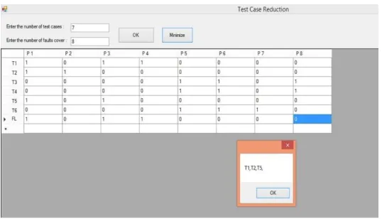
As the result of the work is started to take a program and split it into the predicate based according to their execution of the statement. After that we differentiate the predicate in four parts with its faulty and non faulty statement. To differentiate the predicate we use the Bhattacharya coefficient from their spectrum distribution and then we separate the predicates from inter and intra class distance.The initial step of our model that elaborate how many number of test cases and how many number of fault cover has been entered. Now we perform the test cases reduction technique to reduce the test cases with the coverage matrix based structure to perform the AND operation among the failed test case and the result is then perform with the all passed test cases one by one. First of all entering the values in number of test cases and in number of fault cover and clicking Ok button to get a matrix form of the figure with its test case in rows and cover faults in its columns.

In Figure 8, we give the number of test cases is 7 and the number of fault cover is 8, then clicking Ok button to get coverage matrix and fill all boxes with 0‟s and 1‟s according to their passed and failed statements and the last test case is fault localization requirement vector (FLreq) which is already the AND operation of failed test cases.

5

R

W

There is one of the most famous fault localization technique named as Tarantula [9]. In this technique there proportion of failed and passed execution exercising the statement to measure the dubious part of that statement. Naish et al [14] gave a summary for such technique. Now if we comparing such statement level technique, for locating a fault CBI [10] uses predicates as fault indicator. Which gain low complexity and high extensibility? Zhag et al. [21] empirically validate that the short circuiting has effect the predicate based technique and proposed DES [21] accordingly. They also used a non parametric predicate based statistical fault localization framework.For statistical fault localization there is a well-known impact factor is coincidental correctness which causes program runs and trigger the fault, to be marked as non-failed runs. Test suite reduction is one of a solution [8][15] to address coincidental correctness or improve test suite quality [19], but its feasibility relies on the accuracy of recognizing coincidental cases [13]. Our paper proposes a methodology to address coincidental correctness, which does not rely on the accuracy of recognizing them. In this paper, Bhattacharyya coefficient is used to measure the similarity of the predicate spectra between failed runs and non-failed runs, to rule out the fault-led predicates. After that inter and intra-class distances are often used in pattern recognition to measure the class difference [16,17].

6

C

In this paper we have presented a technique for calculating the fault localization, which is used to locate the fault in a faulty program and give useful solutions for optimization. The program is divided into four types predicates named as Neutral Predicate, Fault Leading Predicate, Fault led Predicate and Balanced Predicate by dynamic spectra. These predicate are distinguish by their dynamic spectra with inter class distance. The program are executed statement wise in every test cases (T1, T2, T3, T4, T5, T6, T7,T8) and prepare a coverage matrix by

their pass and failed test cases in binary form 0‟s and 1‟s. We calculate the fault localization requirement vector (FLreq) by performing AND operation of failed test cases and then performs AND operation between FLreq with each passed test cases to get the weekly irrelevant statement (0000000 or 111111). At the end we reduce the test cases (T1, T2, T5, T7, T8)

where T7 and T8 are already failed test cases and faulty so we

get (T1, T2, T5) as reduce test case.

REFERENCES

[1] P. Arumuga Nainar, T. Chen, J. Rosin, and B. Liblit, Statistical debugging using compound Boolean predicates, Proc. ISSTA ,pp. 5-15, 2007.

[2] Bhattacharyya. On a measure of divergence between two statistical populations defined by probability distributions. Bulletin of the Calcutta Mathematical Society,

[3] T.M. Chilimbi, B. Liblit, K. Mehra, A.V. Nori, and K. Vaswani, HOLMES: effective statistical debugging via efficient path profiling, Proc. ICSE, pp. 34-44, 2009.

[4] W. Dickinson, D. Leon, and A. Podgurski. Pursuing failure: the distribution of program failures in a profile space. Proc. ESEC/FSE, pp. 246-255, 2001.

[5] H. Do, S. G. Elbaum, and G. Rothermel, Supporting controlled experimentation with testing techniques: an infrastructure and its potential impact, Experimentation in Software Engineering, vol. 10(4), pp. 405-435, 2005.

[6] R. Gore, and P. F. Reynolds. Reducing confounding bias in predicate-level statistical debugging metrics, Proc. ICSE, pp. 463-473, 2012.

[7] Y. Guan, H. Wang. Set-valued information systems. Information Sciences, vol. 176(17), pp. 2507-2525, 2006.

[8] D. Hao, Y. Pan, L. Zhang, W. Zhao, H. Mei and J. Sun, A similarity-aware approach to testing based fault localization, Proc. ASE, pp. 291-294, 2005.

[9] J.A. Jones and M.J. Harrold, Empirical evaluation of the Tarantula automatic fault-localization technique, Proc. ASE, pp. 273-282, 2005.

[10]B. Liblit, M. Naik, A. X. Zheng, A. Aiken, and M.I. Jordan, Scalable statistical bug isolation, Proc. PLDI, pp. 15-26, 2005.

[11]C. Liu, L. Fei, X. Yan, S. P. Midkiff, and J. Han, Statistical debugging: a hypothesis testing-based approach, IEEE TSE, vol. 32(10), pp. 831-848, 2006.

[12]W. Masri and R. A. Assi. Cleansing test suites from coincidental correctness to enhance fault-localization, Proc. ICST, pp. 165-174, 2010.

[13]Y. Miao, Z. Chen, S. Li, Z. Zhao, and Y. Zhou, Identifying coincidental correctness for fault localization by clustering test cases, Proc. SEKE, pp. 262-272, 2012.

[14]L. Naish, H.J. Lee, and K. Ramamohanarao, A model for spectra-based software diagnosis, ACM TOSEM, vol. 20(3):11, 2011.

[15]R. Santelices, J.A. Jones, Y. Yu, and M.J. Harrold, Lightweight fault-localization using multiple coverage types, Proc. ICSE, pp. 56-66, 2009.

386

[17]L. Wang, Feature selection with kernel class separability, IEEE Transactions on Pattern Analysis and Machine Intelligence, vol. 30(9), pp. 1534-1546, 2008.

[18]X. Wang, S. C. Cheung, W. K. Chan, and Z. Zhang. Taming coincidental correctness: Coverage refinement with context patterns to improve fault localization. Proc. ICSE, pp. 45-55, 2009.

[19]Y. Yu, J. A. Jones, and M.J. Harrold, An empirical study of the effects of test-suite reduction on fault localization, Proc. ICSE, pp. 201-210, 2008.

[20]Z. Zhang, W.K. Chan, T.H. Tse, B. Jiang, and X. Wang, Capturing propagation of infected program states, Proc. ESEC/FSE, pp.43-52, 2009 .

[21]Z. Zhang, B. Jiang, W. K. Chan, T. H. Tse, and X. Wang, Fault localization through evaluation sequences, Journal of Systems and Software, vol. 84(6), 2010.

[22]Heng Li, Yuzhen Liu (2014) “Program Structure Aware Fault LocalizationState Key Laboratory of Computer Science Institute of Software, Chinese Academy of Sciences Beijing 100190, ChinaNorth China Electric PowerUniversity Beijing 100190, China

[23]Gong Dandan, WangTiantian ,SuXiaohong, MaPeijun (2014) “A test-suite reduction approach to improving fault-localization effectiveness” School of Computer Science and Technology, Harbin Institute of Technology, Harbin 150001, China

[24]Heng Li, Yuzhen Liu, Zhenyu Zhang, Jian Liu (2014) “Program Structure Aware Fault Localization” State Key Laboratory of Computer Science Institute of Software, Chinese Academy of Sciences Beijing 100190, China