https://doi.org/10.5194/tc-11-1333-2017
© Author(s) 2017. This work is distributed under the Creative Commons Attribution 3.0 License.
Sonar gas flux estimation by bubble insonification: application to
methane bubble flux from seep areas in the outer Laptev Sea
Ira Leifer1, Denis Chernykh2,3, Natalia Shakhova3,4, and Igor Semiletov2,3,4 1Bubbleology Research International, Solvang, CA 93463, USA
2Russian Academy of Science, Pacific Oceanological Institute, Vladivostok, Russia 3Tomsk Polytechnic University, Tomsk, Russia
4University Alaska Fairbanks, International Arctic Research Center, Fairbanks, AK 99775, USA Correspondence to:Ira Leifer ([email protected])
Received: 23 June 2016 – Discussion started: 7 July 2016
Revised: 6 February 2017 – Accepted: 6 February 2017 – Published: 9 June 2017
Abstract.Sonar surveys provide an effective mechanism for mapping seabed methane flux emissions, with Arctic sub-merged permafrost seepage having great potential to signif-icantly affect climate. We created in situ engineered bub-ble plumes from 40 m depth with fluxes spanning 0.019 to 1.1 L s−1 to derive the in situ calibration curve (Q(σ)). These nonlinear curves related flux (Q) to sonar return (σ) for a multibeam echosounder (MBES) and a single-beam echosounder (SBES) for a range of depths. The analysis demonstrated significant multiple bubble acoustic scattering – precluding the use of a theoretical approach to deriveQ(σ )
from the product of the bubbleσ(r) and the bubble size distri-bution whereris bubble radius. The bubble plumeσ occur-rence probability distribution function (9(σ )) with respect toQfound9(σ )for weakσwell described by a power law that likely correlated with small-bubble dispersion and was strongly depth dependent. 9(σ ) for strong σ was largely depth independent, consistent with bubble plume behavior where large bubbles in a plume remain in a focused core.
9(σ )was bimodal for all but the weakest plumes.
Q(σ )was applied to sonar observations of natural arctic Laptev Sea seepage after accounting for volumetric change with numerical bubble plume simulations. Simulations ad-dressed different depths and gases between calibration and seep plumes. Total mass fluxes (Qm) were 5.56, 42.73, and 4.88 mmol s−1 for MBES data with good to reasonable agreement (4–37 %) between the SBES and MBES systems. The seepage flux occurrence probability distribution function (9(Q)) was bimodal, with weak 9(Q) in each seep area well described by a power law, suggesting primarily minor
bubble plumes. The seepage-mapped spatial patterns sug-gested subsurface geologic control attributing methane fluxes to the current state of subsea permafrost.
1 Introduction 1.1 Arctic methane
On a century timescale, methane (CH4)is the next most im-portant anthropogenic greenhouse gas after carbon dioxide (CO2)(Forster et al., 2007). However, on a decadal timescale comparable to its atmospheric lifetime, CH4is more impor-tant to the atmospheric radiative balance than CO2(Forster et al., 2007; Fig. 2.21). After nearly stabilizing, atmospheric CH4 concentrations are increasing again, although the un-derlying reasons remain poorly understood (Nisbet et al., 2015). Despite likely increasing future natural emissions from global warming feedbacks (Rigby et al., 2008) and an-thropogenic activities (Kirschke et al., 2013; Wunch et al., 2009), many source estimates have large uncertainties with greater uncertainty in future trends. This is particularly rele-vant for Arctic sources where global warming is the strongest (Graversen et al., 2008).
most extensive sedimentary basin in the world (Gramberg et al., 1983).
Terrestrial Arctic permafrost CH4provides important cli-mate feedbacks (Friedlingstein et al., 2006; Lemke et al., 2007) as does subsea permafrost – submerged terrestrial per-mafrost (Shakhova and Semiletov, 2009). Subsea perper-mafrost degradation drives seabed CH4 bubble emissions. Assess-ing these emissions is challengAssess-ing due to the vast extent of the East Siberian Arctic Shelf (ESAS) seep field (Shakhova et al., 2014; Stubbs, 2010), the world’s most extensive seep field.
Sonar is the most common survey approach and has been used on concentrated seep areas covering ∼1000 m2 in the North Sea (Schneider von Deimling et al., 2007, 2010; Wilson et al., 2015), far more dispersed and weaker seepage in the Black Sea of ∼2500 plumes in an area of ∼20 km2 (Greinert et al., 2010), and offshore Svalbard where a few hundred plumes were observed in an area of
∼15 km2(Veloso et al., 2015). Sonar can also be used from remotely operated vehicles for the deep sea, e.g., Muyak-shin and Sauter (2010) for the Haakon Mosby mud volcano (3 plumes).
Sonar has also mapped significantly larger and stronger seepage in the Coal Oil Point (COP) marine hydrocarbon seep field offshore California. The COP seep field covers
∼3 km2of active seabed in an 18 km2area releasing 105m3 CH4 per day (Hornafius et al., 1999), likely composed of many tens of thousands of plumes. A single survey requires two days (Leifer et al., 2010).
ESAS seepage is on a dramatically larger scale with
∼30 000 plumes manually identified in just two transects (Shakhova et al., 2014; Stubbs, 2010). Seepage densities up to∼3000 seep bubble plumes per km2were found transect-ing a stransect-ingle hotspot. Based on the hotspot size (18 400 km2), an order of magnitude estimate suggests 60 million seep plumes for the hotspot alone. Two sonar survey transits of the ESAS required a month.
1.2 Study motivation
Given the ESAS seepage extent there is a critical need for new approaches to effectively, rapidly, and quantitatively sur-vey seepage areas. Video is inadequate to sursur-vey extensive or widely dispersed seepage, a task for which sonar (active acoustics) excels. This study demonstrates an improved ap-proach to quantify seabed seepage using in situ calibrated sonar-derived bubble fluxes. Bubble plumes were observed in the ESAS and offshore California. In combination, the in situ studies covered a broad range of flows and included fine-depth resolution of near-source (growth) plume processes (California) and coarser resolution of plume processes to tens of meters where the plume is self-similar.
Both multibeam echosounder (MBES) and single-beam echosounder (SBES) data were collected in the ESAS, just MBES data of rising engineered bubble plumes were
col-lected in California. These data were colcol-lected both as a depth-dependent calibration and to investigate the effect of multiple acoustic scattering in bubble plumes.
The calibration was applied to quantify in situ sonar obser-vations of three natural seepage areas in the ESAS. Because the calibration bubble plumes and seep bubble plumes were different gases and from different source depths, bubble dis-solution rates are different – i.e., for the same seabed mean volume flux, the depth-window-averaged volume fluxes are different. We demonstrate a first correction attempt based on a numerical bubble plume model between the calibration and natural seepage bubble flows.
1.3 The East Siberian Arctic Shelf
The Siberian Arctic Shelf contains vast CH4 deposits as subsea permafrost, CH4 hydrates, and natural gas reser-voirs (Gautier et al., 2009; Gramberg et al., 1983; Ro-manovskii et al., 2005; Serreze et al., 2009; Shakhova et al., 2010a, b; Shakhova and Semiletov, 2009). Reservoir estimates are∼10 000 Gt (1 Gt=1015g) of CH4 hydrates (Dickens, 2003). Remobilization of even a small fraction of this CH4 could trigger abrupt climate warming; Archer and Buffett (2005) estimated that atmospheric release of just 0.5 % of the Arctic shelf hydrate CH4could cause abrupt cli-mate change.
The ESAS is the world’s largest and shallowest shelf (covering 2.1×10⁶km2)containing the largest area of sub-merged permafrost by far (Shakhova et al., 2010a, b). The ESAS is a seaward extension of the Siberian tundra that was flooded during the Holocene transgression 7–15 kyr ago (Ro-manovskii et al., 2005). The ESAS comprises∼25 % of the Arctic continental shelf and contains over 80 % of global subsea permafrost and shallow hydrate deposits, estimated at ∼1400 Gt carbon (Shakhova et al., 2010a). This reser-voir includes hydrate deposits of∼540 Gt of CH4 with an additional two-thirds (∼360 Gt) trapped below as free gas (Soloviev et al., 1987).
Permafrost degradation
ESAS subsea permafrost degradation allows the release of sequestered CH4 to the shallow ocean and atmosphere and has been changing in response to glacial and interglacial Arc-tic warming (∼7◦C) and warming from the overlying sea-water (∼10◦C) since inundation in the early Holocene with additional ESAS seawater warming in recent decades (Bias-toch et al., 2011; Semiletov et al., 2013, 2012; Shakhova et al., 2014).
submerged offshore permafrost (Romanovskii et al., 2005). Recent observations of offshore permafrost (Shakhova et al., 2014) show that the ESAS permafrost lid is perforated, with year-round CH4 emissions to the atmosphere coming from the sedimentary reservoir (Shakhova et al., 2010a, 2015). This migration feeds a vast marine seep field entirely in shal-low waters where emissions contribute directly to the atmo-spheric budget (Shakhova et al., 2014).
There are important geologic controls on the subsea per-mafrost’s thermal state. On millennia timescales, increasing temperatures of the overlying bottom seawater affect subsea permafrost through heat transfer and salinization (Shakhova et al., 2014, 2015; Soloviev et al., 1987). Geologic con-trol also arises from heat transport by large Siberian rivers, which drives bottom water warming and is proposed to con-trol the distribution of open taliks in coastal ESAS waters (Shakhova et al., 2014). Global warming enhances terrestrial riverine heat including from ecosystem responses, degra-dation of terrestrial permafrost, and increased river runoff. Warm riverine runoff drives a downward heat flux to shelf sediments and subsea permafrost (Shakhova and Semiletov, 2007; Shakhova et al., 2014).
Heat flow in rift zones also provides geologic control (Drachev et al., 2003; Nicolsky et al., 2012). High heat flow areas include relic thaw lakes and river valleys that were sub-merged during the Holocene inundation. These still drive modern permafrost degradation (Nicolsky and Shakhova, 2010; Nicolsky et al., 2012; Shakhova and Semiletov, 2009). Subsea permafrost degradation is greatest in the outer shelf waters (deeper than 50 m) where submergence occurred first, such as the outer Laptev Sea where models predict mostly de-graded permafrost (Bauch et al., 2001). Riverine input to the Laptev Sea also supports the formation and growth of sub-sea thaw lakes and taliks, which are effective gas migration pathways to the seabed (Hölemann et al., 2011; Nicolsky and Shakhova, 2010; Shakhova and Semiletov, 2007; Shakhova et al., 2014).
Active seafloor spreading in the Laptev Sea, which is un-dergoing continental rifting, leads to strong geologic heat flow (85–117 m W m−2). The outer Laptev Sea is one of the few places where active oceanic spreading approaches a con-tinental margin (Drachev et al., 2003) and correlates with the “hot” area crossed by the Ust’ Lensky Rift and Khatanga-Lomonosov Fracture (Drachev et al., 2003; Nicolsky et al., 2012). Evidence of rifting is provided by hydrothermal fauna remnants documented around grabens (dropped blocks be-tween faults) in the up-slope area that typically occurs along oceanic divergent axes (Drachev et al., 2003). Grabens in the ESAS are often linear structures that correlate spatially with paleo-river valleys.
1.4 Marine seepage fate and bubble processes
Marine seepage is a global phenomenon where CH4 and other trace gases escape the seabed as bubbles that rise
to-wards the sea surface (Judd and Hovland, 2007). These bub-bles dissolve and deposit CH4 in the water column, trans-porting their remaining contents to the sea surface – if they reach it (Leifer and Patro, 2002). The fate of these bubbles and their gas depends strongly on depth, size (Leifer and Pa-tro, 2002), flow strength – plume synergies that include the upwelling flow velocity (VZ; Leifer et al., 2009), and bub-ble surface properties like contamination (Leifer and Patro, 2002).
The fate of dissolved seep CH4depends most strongly on its deposition depth (Leifer and Patro, 2002) with CH4 be-low the winter wave mixed layer (WWML) largely oxidized microbially (Rehder et al., 1999). In the shallow Coal Oil Point seep field, most of the CH4reaches the atmosphere di-rectly (Clark et al., 2005) from mixing in the near field (Clark et al., 2000) and in the far (down-current) field when winds strengthen as typically occurs diurnally for coastal Califor-nia. The same is true for the shallow ESAS where virtu-ally all seabed CH4(dissolved and gaseous) is emitted in the WWML and escapes to the atmosphere directly by bubbles or through air–sea gas exchange by frequent storms (Shakhova et al., 2014). Even for deep-sea seepage (to∼1 km), field studies show seep bubble plume CH4transport to the upper water column and atmosphere (MacDonald, 2011; Solomon et al., 2009) from plume processes and hydrate skin effects (Rehder et al., 2009; Warzinski et al., 2014).
Bubble size is important with most seep bubbles in a nar-row range. Based on a review of 39 bubble plume size distri-butions (the most comprehensive published dataset to date), Leifer (2010) found that the vast majority of reported seep bubble plumes could be classified in two categories termed major and minor, with minor being the most common – see also the studies reviewed in Leifer (2010). Bubble plume size distributions (8(re)) for minor bubble plumes are well described as Gaussian and largely composed of bubbles in a narrow size range, 1000< re<4000 µm, where re is the equivalent spherical radius. Major bubble plumes generally escape from higher-flow vents with a power law size distri-bution (Leifer and Culling, 2010). Most major bubble plumes are small, down tore<100 µm; however, plume volume is primarily found in the largest bubbles, up tore∼1 cm (Leifer et al., 2015b).
1.5 Sonar seep bubble observations
Seep 8(re) have been measured by video (Leifer, 2010; Römer et al., 2012; Sahling et al., 2009; Sauter et al., 2006) and passive acoustics. Passive acoustic8(re) measurement has only been demonstrated for low-flow bubble plumes where the individual bubble acoustic signatures can be iden-tified (Leifer and Tang, 2006; Maksimov et al., 2016).
re-solved by MBESs. Additionally, sonar (SBES or MBES) loses fidelity from multiple plumes in close proximity (Schneider von Deimling et al., 2011; Wilson et al., 2015) where the sonar returns along multiple pathways, creating ghosts, shadow noise, off-beam returns, scattering loss, and other artifacts (Wilson et al., 2015). Note that if bubble spa-tial densities are sufficiently high for artifacts to occur be-tween plumes, then the bubbles inside the plumes will pro-duce artifacts inside the plumes. The vessel acoustic environ-ment can be noisy and signal loss from scattering can also occur from suspended sediment and biota, often in layers.
There are many challenges to the quantitative derivation of bubble emission flux from sonar return, which at its basis relates to the interaction of sound with a bubble. For a single spherical bubble, the relationship has long been known with resonance given by the Minnaert (1933) equation:
fo= 1 2π re
3γ P
ρ
1/2
, (1)
wherefo is the resonance (or Minnaert) frequency,γ is the polytropic coefficient,P is internal bubble gas pressure, and
ρ is pressure. This is the frequency a bubble emits at for-mation. For nonspherical bubbles (re>150 µm) there is an eccentricity correction based on the bubble-axis-wave front angle. Bubble eccentricities vary from 1.0 for spherical bub-bles to 2 or greater forre>3500 µm (Clift et al., 1978). For a single spherical bubble, the back-scattering cross section (σ )
nearfois (Weber et al., 2008)
σ = r
2 e
fo f
2
−1 2
+δ2
(2)
wheref is the frequency andδis the damping term, approxi-mated asδ∼0.03f0.3withfin kHz. For bubbles larger than resonance, σ varies within 5 or so dB; for bubbles smaller than resonance, it decreases precipitously – 35 dB for a fac-tor of 2 decrease inre (Weber et al., 2014). Integrating over the bubble emission size distribution, which is the number of bubbles in are bin, passing through the measurement plane combined with the bubble vertical velocity (VZ(re)), which is a function of reover the measurement volume yields the total plume cross section if bubbles are acoustically non-interfering (no multiple scattering) and the bubble–sonar in-teraction is isotropic – i.e.,σBis independent of angle despite bubble eccentricity.
However, bubbles are often clustered in close proximity in seep bubble plumes, which allows multiple scattering be-tween bubbles that decreasesσ significantly (Weber, 2008). Acoustic modeling of bubble clusters is complicated even for small spherical bubbles – e.g., see Weber (2008). Specif-ically, σ depends on 8(re, x, y, z) in the plume, which is asymmetric with respect to currents and evolves as the bubble plume rises. Acoustic propagation across a plume varies with
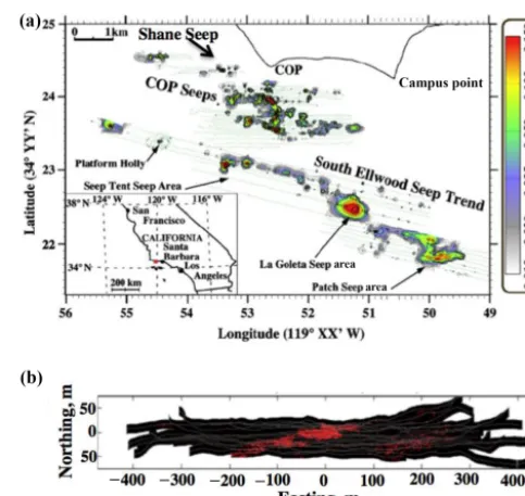
Figure 1. (a)Coal Oil Point (COP) seep field map showing the Shane Seep area of the scoping study. Sonar data from 2005 was adapted from Leifer et al. (2010).(b)Shane Seep multibeam sonar survey map of seep detection (2 m depth window at a seabed-following height of 4 m). MBES data was collected in 2009.
azimuthal angle because bubbles are compressible, leading to different bubble–bubble acoustic interactions. Bubble ec-centricity also contributes an azimuthal angle dependency. Whereas artifacts, like ghosting, between plumes (not side lobe return) can be spatially segregated, this is not feasi-ble for such artifacts inside the plume. Here the bubfeasi-bles are within a few centimeters (∼10–20re)of each other, such as bubbles in the wake of a larger bubble (Tsuchiya et al., 1996) and near the seabed, acoustic coupling leads to frequency shifts (Leifer and Tang, 2006) that decreaseσ.
2 Methodology 2.1 Field study areas
This study reports on the use of in situ engineered plumes for calibration ofσ to derive quantitative flux rates using a MBES which was deployed in the Coal Oil Point seep field, offshore California in the northern Santa Barbara Channel, in the Kara Sea of the ESAS. We present the small fraction of collected Kara Sea and ESAS data that were cleared for publication.
2.1.1 Coal Oil Point seep field
de-ployed∼15 m from the center of Shane Seep, which covers an area of∼104m2in∼20 m water depth and comprises on the order of 1000 individual vents or bubble plumes (Fig. 1b). The lander included a MBES (Delta T, Imagenex, Vancouver, Canada) and compass (Ocean Server, MA) on an underwa-ter rotator (Sidus Solutions, CA) with an azimuthal rotation angle range of up to 270◦. The sonar produced a 260 kHz vertically-oriented 128-beam fan spanning 120◦ tilted up-wards to reduce seabed backscatter. Two in situ calibration air bubble flows were deployed ∼8 m from the lander at azimuthal angles beyond the active seepage area and were traversed during each sonar rotation cycle. Two rotameters measured regulated airflows from an onboard compressor to these two bubble plumes.
2.1.2 Arctic field campaign
Field data were obtained during an expedition onboard the R/VViktor Buynitsky from 2 September to 3 October 2012 (Figs. 2 and 3). TheVicktor Buynitskysailed from Murmansk to the Laptev Sea and the adjacent portion of the ESAS. The expedition’s overarching goal was to improve the un-derstanding of the current scale of ESAS CH4 emissions in order to develop a conceptual model of CH4 propaga-tion from the seabed to the atmosphere, including assessing source strengths and their dynamics.
The calibration experiments were conducted in a region of no natural seepage and almost flat seafloor in the Kara Sea (Fig. 3) to reduce or eliminate off-beam acoustic seabed scattering. Water depth was 45 m and weather was favor-able: calm sea with a wind speed of 1–3 m s−1 and wave height of 0.2–0.5 m with no significant waves (0 to 1 ball). Column profile temperature and salinity data were measured using a conductivity, temperature, and depth (CTD) profiler (SBE19+, Seabird, USA). Weather for the seep sonar survey was typical (3–4 storm events with wind speed>10 m s−1). The vessel was anchored during the engineered bubble plume experiments. Engineered bubble plumes were made from nitrogen supplied by a pressure tank on the vessel fore-deck. A 70 m long, 12 mm diameter, 6 mm wall thickness gas supply tube was attached by a Kevlar rope to a heavy metal weight (∼30 kg) that ballasted against buoyancy of gas in the tubing and drag from currents. The supply tube was de-ployed to a 40 m depth (Fig. S3) and the rising bubble plume was observed with a MBES and SBES. The sonars were lo-cated near each other so that their beam coverage overlapped with the center beam focused on the end of the bubble stream. Bubbles were produced from a 4 mm diameter copper nozzle attached at the end of the gas supply tube.
Gas flow was controlled using standard flow meters. One port was connected to a PVC tube and a second port was connected to a two-way valve. The third port was connected to the gas tank through the gas manifold. The manifold con-sisted of a high-pressure sensor for the tank pressure and a low-pressure sensor for the outgoing pressure (5.5 bar). We
used temperature-compensated differential-pressure sensors with a manufacturer-specified range of±1 psi (equivalent to
±70 cm of water). The sensor has a manufacturer-specified accuracy and stability of±0.5 % FSD (full scale deflection over the operating-pressure range of the sensor over one year, between 0 and 50◦C) and repeatability errors of ±0.25 % FSD. For the study, the gas flow was varied from 0.5 to 150 L min−1at 5.5 bar (equal to the bubble outlet hydrostatic pressure). For each experiment, the gas flow was allowed to stabilize and then sonar data were recorded for∼10 min.
The same MBES was used in the ESAS and COP seep field. The SBES was a SIMRAD EK15 SW 1.0.0 echosounder (http://www.simrad.com) at 200 kHz, with a 1 ms pulse duration at 10 Hz, a 26◦ beam width, and a built-in calibration system. Sonar data, including seep bub-ble plumes, were recorded at an average survey speed of 4–6 knots. Sonar backscatter was calibrated using acoustic targets (SIMRAD, Denmark). Initial data visualization and process-ing used EchoView and Sonar 5 software (SIMRAD) for the EK15 echosounder.
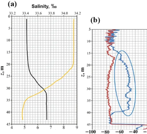
Bubbles have high density contrast with water and thus are strong sonar targets that can be distinguished easily from the background (Fig. 4b). For the engineered bubble plume ex-periments, the wave-mixed layer (WML) extended to∼35 m depth with upper water∼3.5◦C warmer than deeper water (Fig. 4a).
Sonar data analysis and visualization was performed with custom MATLAB routines (MathWorks, MA) that first geo-rectified each ping and then assembled the data for each ex-perimental run into a three-dimensional array of depth (z), transverse distance (x), and along track distance (y) or time (t) if stationary.
2.2 Seep and engineered bubble plume modeling A numerical bubble propagation model was used to explore the relative dissolution rates for seep versus calibration bub-ble plumes and to calculate a volumetric correction factor that accounted for the difference. The bubble model is de-scribed elsewhere (Leifer et al., 2006; Leifer and Patro, 2002; Leifer et al., 2015b; Rehder et al., 2009). The model solves the coupled differential equations describing bubble molar content (Eq. 3), size (Eq. 4), pressure, and rise for each bub-ble size class in a bubbub-ble plume. These equations describe how sonar observations of bubble volume (size) relate to bub-ble mass (molar content).
Bubble dissolution or gas flux (Fi)for each gas species (i) is the change in bubble molar content (ni)with time (t) driven by the concentration difference(1Ci) between the bubble and the surrounding water:
Fi=
∂ni
∂t =kBiA (1Ci)=kBiA (Ci−HiPi) , (3)
Figure 2.Map for the R/VViktor Buynitskycruise, 2012.
Figure 3.Locations of oceanographic stations for the RVViktor Buynitskycruise, 2012, marked by yellow circles. Polygons of major focus areas are marked as P1 (northern Laptev Sea), P2 (east Lena Delta), and P3 (Dmitry Laptev Strait) shown in insets. Ship tracks accompanied by CTD (conductivity, temperature, and depth) measurements (and geophysical surveys) performed in the P1 are shown as red lines.
area,His the Henry’s Law equilibrium, andP is the bubble partial pressure. Seep gases, such as CH4, largely outflow (positiveF) while air gases inflow (negativeF).
Fi depends on depth andrethroughkBand alsoA(Leifer and Patro, 2002). Deeper bubbles of the same re contain greater mass, allowing for longer survival and rise. Seep bubbles are seldom isolated (Leifer, 2010); thus, plume pro-cesses are important, including the upwelling flow which de-pends on the total plume volume flux (Leifer et al., 2009; Leifer et al., 2006). Another plume process is enhanced aque-ous concentrations relative to the surrounding water, which
enhances bubble survival (Leifer et al., 2006):
∂re
∂t =
RT∂n
∂t −
4π re3
3 ρWg
∂z ∂t 4π r
2
PA−ρWgz+ 2α
re
−4π r
3
3 2α
r2 e
−1
, (4)
wereR is the universal gas constant,T is temperature, and
Figure 4. (a)Salinity and temperature (T) with respect to depth (z) during engineered bubble plume experiments.(b)Single-beam echosounder sonar return integrated across the plume (σ) withzfor a bubble plume (blue) and for no bubble plume (red); the bubble plumeσ is circled.
Figure 5. (a) Minor bubble plume size distribution (8)with re-spect to the equivalent spherical radius (r) used to initialize the bub-ble model.(b)Measured temperature (T)-depth (z) profile used in model.
Unfortunately, bubble size distributions were not mea-sured, and thus a typical minor bubble size distribution from the literature was used. Implications of these simplifying as-sumptions are discussed in Sect. 4.4.
The model was initialized with a typical (Leifer, 2010) minor 8 (Fig. 5a) for either methane or nitrogen bubbles, dissolved air gases at equilibrium in the water column, the observed CTD profile (Fig. 5b), and a 10 cm s−1upwelling flow.VZ is an average value that is too low for the highest calibration flow and too high for the lowest (Leifer, 2010).
Figure 6.Field sonar data from the Coal Oil Point seep field for air bubbles in 22 m deep water. Sonar return counts integrated across the plume (σ) versus airflow (Q) and height above seabed (h) for four airflows and least-squares linear regression fits to log(σ )versus
h.
3 Results
3.1 Engineered bubble plumes
Sonar return for the two (high and low) calibration plumes (Fig. S2) was thresholded above background (bubble-free water) and integrated for each beam during rotation across each calibration plume. The thresholdedσ in a depth win-dow then was fit with a linear polynomial of the log of the integrated sonar return over the plume versus height (h). As the bubble plume rose,σ increased – i.e.,σ (h) was not con-stant (Fig. 6). Note, the change in volume for air bubbles over such short rise heights is negligible. This is evidence of decreasing bubble–bubble acoustic interaction as the bub-bles rise and spread from turbulence (acoustic interactions decrease towards zero as the inter-bubble distances increase). Note that these data were uncalibrated and cannot be directly compared to the Arctic calibration data; this is presented to show the depth trends.
There is significant geometric uncertainty in SBES data, which is evident in the overlap in time of sonar returns for the calibration bubble plume (Fig. S4). This overlap results from current advection of the plume orthogonal to the page. MBES addresses this SBES deficiency. For example, the SBES loses the bubble plumes once they have risen into the WML, where currents often shift, but the MBES continues to observe them to 13 m depth, slightly below the vessel’s draft.
The most common sonar return ping element is noise, which was isolated from the bubble plume signal by setting a threshold from the sonar return probability distribution func-tion (9(σ )) at approximately−80 dB (Fig. 7a). The 9(σ )
(Fig. 7a, arrow), which provided a 5–8 dB transition between noise and bubbles. Obvious sonar artifacts, which can exhibit strong sonar return signatures, were masked by spatial segre-gation. Specifically, the plume center was identified at each depth and then filtered to ensure continuity with depth. Then, only samples within a specified horizontal distance from the plume centerline that tightly constrained the plume above the noise threshold were incorporated into the analysis.
For the engineered bubble plume experiments, plumes with volume flux (Q) from 0.019 to 1.1 L s−1were created and observed by both SBES and MBES systems (Fig. 7). The contribution of bubble plume weak and strong sonar returns were investigated by their signature in 9(σ ). Specifically,
9(σ ) was modeled by a piecewise least-squares linear re-gression analysis of 9(σ )=aσ (z)b. This model was then compared to expected trends in plume evolution of a rising bubble plume. Fit parameters are shown in Table S1 in the Supplement. Example data and fits for the 0.8 L s−1 plume shown in Fig. 9d–f for three depth windows (all below the WML).
For low- versus high-flow plumes, 9(σ ) was distinctly different, whereas9(σ )for the intermediate-flow plume ex-hibited characteristics of both low and high flows. A weak
σ represents small bubbles, whereas a strong σ may re-flect large bubbles or dense aggregations of small and/or large bubbles. As a bubble plume rises, the relative impor-tance of small bubbles should increase as small bubbles dis-perse, spreading the weak sonar return over a larger volume.
9(σ ) at the deepest depth for the weakest bubble plume exhibited a clear, two-part power law (Fig. 7c; Table S1) and remained constant as the bubble plume rose for the first 10 m, abruptly steepening in the next 5 m. This emphasizes the importance of smaller bubbles (b= −8, −7, and −12 for weak σ for the 45–40, 40–35, and 35–30 m depth win-dows, respectively). For the weaker bubble plumes (0.042 and 0.019 L s−1, Fig. 7b and c, respectively), the strongest
σ disappear completely at the shallowest depth, consistent with bubble plume dispersion, bubble dissolution, and strong currents.
9(σ ) is bimodal for the deepest depth window for the highest-flow plume (Fig. 7d) with strongerσ more common relative to weakerσ than in the low-flow plume (Fig. 7c) and more common than “predicted” by extrapolating the weak
σ power law fit (σ−10.7)to stronger σ (Fig. 7d and f, re-spectively). As this plume rose,9(σ )for weakσ decreased in relative importance while 9(σ )for strongerσ remained constant. The power law exponent for the intermediate depth (b= −7.4) was less steep than for deeper (−10.7) and shal-lower (−8.4) depths. Thus, most of the evolution of9(σ )
is from spatial expansion of weakerσ, i.e., smaller bubbles, while the denser, stronger σ bubbles remain relatively uni-formly constrained with depth. The overall increase in σ
with rise exhibits the same depth evolution as observed in the precursor COP study (Fig. 6) which featured strong plumes comparable to the strong plumes in Fig. 7d–f.
9(σ ) for the intermediate-flow plume (Fig. 7b) shares characteristics of both the high- and low-flow plume9(σ )
– bimodal at the deepest depth with a pronounced strongσ
peak in9(σ ), like the high-flow plume, and evolving into a dual power law as the plume rises, as for the low-flow plume
9(σ ). Thus,9(σ )for the intermediate-flow plume evolved as it rose through the patterns of the strong to the pattern of the weak flow plumes.
These are point source plumes that disperse as they rise, thus bubble–bubble multiple scattering should decrease with height. With the exception of the strongest plume, plume rise decreasesσ; however, for the strongest flow plume, rise ini-tially increases σ, similar to the behavior in the precursor study (Fig. 6) which was for comparably high flows albeit over depths much closer to the source. See Figs. S5 and S6 for sample MBES data for these flows.
The depth-dependent calibration curves (σ (Q, z)) were derived to account for the depth-evolving bubble–bubble acoustic interactions as the bubbles rose (Fig. 8). Specifically,
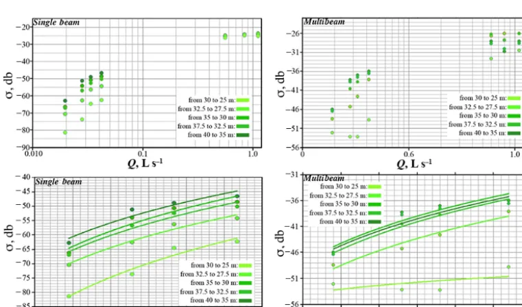
σ above the noise threshold in spatially segregated boxes in each depth window is averaged over 7 min of sonar data for each flow to deriveσ (Q, z). The MBES and SBES calibra-tion datasets show saturacalibra-tion at high flow, similar to Greinert and Nützel (2004), which is evidence of bubble–bubble mul-tiple scattering as shown in simulations by Weber (2008). For the high-flow cases, this likely includes sonar shadowing of more distant bubbles by nearer bubbles (decreasing σ ). At low flow,σ increases with increasingQfar faster than the linear addition of the number of bubbles. For example, for a flow doubling (Q=0.02 to 0.04 L min−1),σshould increase by 20 log10(2), or 6 dB, yet increases are much larger.
σ (Q, z)shows a depth dependency inσfor both SBES and MBES systems (Fig. 8). For low-flow plumes,σ decreases with rise and is nonlinear withQ. In contrast, for high flows, both SBES and MBES systems saturate or are near satura-tion although there is significantly more variability in the MBES data. Saturation occurs when increasedQhas a min-imal to no increase inσ. Close inspection of the high-flow plume MBES data revealed undulations, which may have led to depth aliasing ofσ in the 5 m depth windows. Although the high-flow calibration plumes are relevant for major seep bubble plumes such as in COP seep field (Leifer, 2010), the ESAS plumes studied were weaker. Thus, the strong calibra-tion plumes are not discussed further. In contrast, the low-flow calibration plumes are comparable to typical minor bub-ble plumes (Leifer, 2010) and span the observed range of nat-ural seepage in the study area.
3.2 Bubble dissolution rates and volume flux
Figure 7.Plume-integrated sonar return (σ )occurrence probability distribution function (9(σ ))normalized to sonar bin-width (sonar bins are logarithmically spaced) for(a)full water column for a flow (Q) of 0.8 L s−1– un-thresholded for processed depth windows (z) arrow shows noise threshold;9(σ )is thresholded for(b)Q=0.042 L s−1,(c)0.019 L s−1, and with linear fits forQ=0.8 L s−1for(d)z=35– 40 m,(e)30–35 m, and(f)25–30 m. Data key is on the figures. Fit parameters are in Table S1 in the Supplement.
Figure 8.Sonar return (σ )versus volumetric flow (Q) calibration curves for the single-beam sonar for(a)allQand(c)lowQand for the multibeam sonar for(b)allQand(d)lowQ. Fit parameters are shown in Table S2.
(70 versus 40 m) and different gas composition (seep gas was primarily CH4, while the calibration gas was nitrogen). Both these factors have non-negligible implications for the bubble dissolution rates of the two different plumes.
These differences cause different bubble plume evolution and thus different volume height profiles. A volumetric cor-rection factor was developed based on the ratio of the volume
height profiles between a calibration and a seep bubble plume (same bubble size distribution) based on numerical bubble propagation model simulations (Fig. 9).
pres-Figure 9. (a)Depth (z) evolution of the bubble plume size distribution (8)for a nitrogen minor plume (calibration) from 40 m and(d)for a CH4seep plume from 70 m. Seabed normalized volume averaged over depth window (< Q >) of the rising bubble plume for the(b) calibra-tion plume and(e)seep plume. Molar vertical flux for(c)calibration plume, and(f)seep Data keys on panels.
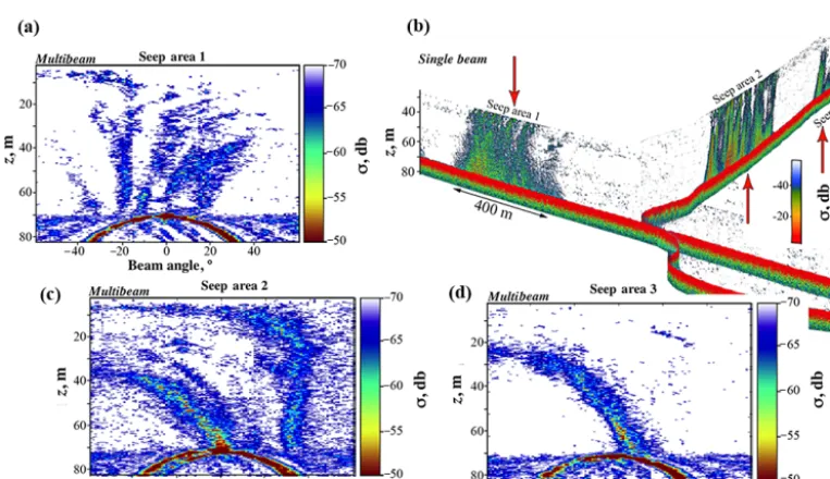
Figure 10.Sonar return (σ) with depth (z) of seep bubble plumes in the Laptev Sea.(a, c, d)Multibeam sonar data, single ping, in each of the seep areas, locations labeled on(b).(b)Single-beam sonar data. The size scales and data keys are shown on the panels.
sure and secondarily from oxygen inflow, while it shrinks from nitrogen outflow. Growth indicates that the balance fa-vors hydrostatic over nitrogen outflow.
The size distribution of a minor seep bubble plume changes dramatically as it rises from a 70 m depth, with the smallest bubbles dissolving and the largest bubbles growing (Fig. 9d). Overall, air uptake and decreasing hydrostatic pres-sure largely balance dissolution for the first 50 m of bubble rise and < Qz> remains roughly stable (Fig. 9e); Q de-creases by 0.7, 0.2, and 0.0 % in the first three 5 m depth
windows. Note that stableQdoes not imply constant total CH4 bubble content, which continually outflows the rising bubble.
Combining the volumes from the two simulations provides the volume correction factors, 0.948, 0.868, and 0.775 for the 65–70, 60–65, and 55–60 m depth windows, respectively. Thus, the calibration plumeQaveraged over the 35–40 m depth window is∼5 % greater than the seep bubble plume
Figure 11.Seep mass flux (Qm)map for(a)all seep areas and for(b–d)Seep areas 1–3. Data key is shown on panel(c).
3.3 Natural seepage
The calibration function (σ (Q, z)) was applied to MBES and SBES Laptev Sea sonar data under strong-current conditions. Flux for the seep areas (Fig. 10) was mapped by averag-ing the seepage flux in the 65–70 m depth window in 1 m2 quadrats after the application of the calibration function and the volume correction factor. The deepest depth window was chosen to better preserve the seabed location of emissions for spatial analysis. Three seep areas were surveyed, two weak and one strong, and all with numerous plumes. The MBES data illustrates the additional spatial information missing in SBES systems. For example, Seep area 1 in the SBES data (Fig. 10b) appears to show extensive diffuse seepage, which the MBES data (Fig. 10a) reveal arises from many low-flow discrete bubble plumes.
Seep area 2 was stronger than the other seep areas by an or-der of magnitude and clearly showed a northeast–southwest trend, which is apparent in all seep areas. Some of the stria-tion patterns, primarily of the weaker returns, are consistent with the very strong currents detraining small bubbles out of the plume in the direction of the sonar beam fan. On a sec-ond, east–west leg, Seep area 1 was surveyed with currents not aligned with the sonar beam fan and does not exhibit stri-ation. Further evidence of the effect of currents is shown in the sonar ping data (Fig. 10b vs. 10c and d), where Seep area 1 does not show the extreme tilt across beams as sonar data for Seep areas 2 and 3. Thus, the linear seep trends reflect geological control.
Seepage spatial structure showed numerous seeps clus-tered around the strongest seep with an apparent modu-lation at distances of ∼125–150 m (Fig. S7). The dom-inant plumes in Seep areas 1 and 3 were as strong as 0.3 mmol m−2s−1 (7.4 cm3s−1) while the dominant seep
plumes in the larger Seep area 2 (Fig. 11c) released
>0.6 mmol m−2s−1(15 cm3s−1).
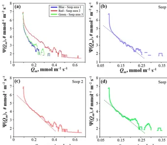
The mass flux (Qm) occurrence probability distribution function (9(Qm)) was calculated for each seep area and showed that Seep area 2 contained the largest number of strong seep plumes followed by Seep area 3 and then Seep area 1 (Fig. 12). For the seep areas, 9(Qm) for weak emissions asymptotically approached ∼0.1 mmol m−2s−1 (2.5 cm3s−1) – the noise level. Thus, calibration flows (Fig. 8) were bracketed from the MBES data from the noise floor to the largest observed seep plume.
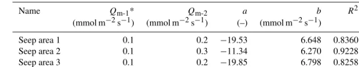
Seep area 2 exhibits both greater fluxes and a shallower power law than other seep areas (Fig. 12c). Furthermore, all seep areas exhibited positive anomalies or peaks in9(Qm) for stronger flux seepage. These peaks signify a preferred emission mode – i.e., multiple seeps with similar emission fluxes. For weaker seeps with good signal to noise ratios (Qm>0.15 mmol m−2s−1), the power law fits are nearly identical: 6.65, 6.27, and 6.80 for Seep areas 1, 2, and 3, re-spectively (Table 2).
Total flux in each seep area was determined by area in-tegration and was 5.56, 42.73, and 4.88 mmol s−1 for the MBES data (Table 2). SBES-derived emissions were biased lower compared to MBES, by 3.7 to 36 % for the seep areas, with best agreement for Seep area 2.
4 Discussion
4.1 Bubble–bubble acoustic interaction
Figure 12. Seep mass flux (Qm) occurrence probability distribution function (9(Qm)) normalized to flux bin-width (bin widths are logarithmically-spaced) for(a)all seep areas and for(b–d)Seep areas 1–3 with power law fits. Data key is shown on panel(a). See Ta-ble 2 for fits.
Table 1.Integrated depth-windowed methane flux estimates.
Designation Qm−SBESa Qm−SBES Qm−MBESb Qm−MBES Area E Qm (mmol m−2s−1) (mmol s−1) (mmol m−2s−1) (mmol s−1) (km2) (%) (L s−1)
Seep 1 0.22 3.78 0.33 5.56 0.017 32 0.14
Seep 2 0.59 41.16 0.61 42.73 0.070 3.7 1.07
Seep 3 0.26 3.96 0.33 4.88 0.015 19 0.12
Qis volume flux,Qmis mass flux, andEis bias, whereE=(Qm-MBES−Qm-SBES)/Qm-MBES.aSBES – single-beam echosounder, 65–70 m, depth window.bMBES – multibeam echosounder, 65–70 m, depth window.
This range was comparable from typical low-flow minor plumes to very strong high-flow major plumes (Leifer, 2010). Calibration plume sonar return increased strongly and non-linearly with flux, ∼15 dB for a flow doubling from 0.02 to 0.04 L s−1. This increase is faster than the 6 dB increase that would be expected by simply summing the sonar cross sections of the doubled number of bubbles. Instead, the increase suggests strong bubble–bubble acoustical interac-tions. Specifically, with increased flow, overall plume dimen-sions expand more quickly, leading to less bubble shadow-ing and shallower sonar occurrence probability distribution function slopes at the same height above the nozzle (Fig. 7). In contrast to the overall plume dimensions (which includes smaller, more-dispersed bubbles), the dense core of large
Table 2.Fit parameters for the seep area flux probability distribution function.
Name Qm-1* Qm-2 a b R2
(mmol m−2s−1) (mmol m−2s−1) (–) (mmol m−2s−1)
Seep area 1 0.1 0.2 −19.53 6.648 0.8360
Seep area 2 0.1 0.3 −11.34 6.270 0.9228
Seep area 3 0.1 0.2 −19.85 6.798 0.8258
Fit fromQm-1toQm-2, whereQmis the mass flux rate.
As a high-flow bubble plume rises, the weak σ portion of the plume representing small bubbles disperses, leading to an increase in the integrated σ as was observed in the Coal Oil Point and ESAS engineered plume data. In the COP seep field study, calibration flows extended from compara-ble to far higher flows than those in the ESAS and docu-mented thatσ (z) increased with height on fine-depth scales (Fig. 6). This was interpreted as due to decreasing bubble “shadowing” of more distant bubbles as the plume expands and becomes more diffuse during the plume growth or ac-celeration phase (Leifer et al., 2015a). As the ESAS calibra-tion plumes rose, the sonar occurrence probability distribu-tion funcdistribu-tion showed a strong influence from small-bubble dispersion as the plume expanded and an increase in the in-tegratedσ (Fig. 8)
As low-flow calibration plumes rise and disperse, σ de-creases. Overlapping intermediate depth windows were eval-uated and confirmed that this was not an artifact of plume os-cillatory motions aliasing the return signal across the depth windows. The decrease in integratedσwith rise is (by defini-tion) a decrease in scattered sonar energy, i.e., greater energy scatters back to the sonar when the plume is spatially denser. This could arise from a decrease in shadowing from scatter-ing or dissolution; however, the bubble model showed that minor plume dissolution did not change overall plume vol-ume significantly (Fig. 9), unlike the significant changes in integratedσ(e.g., Fig. 8c).
4.2 Bubble detrainment and bubble–bubble acoustic interaction
The artifact striations in the natural seep sonar data from currents are consistent with a non-negligible bubble–bubble acoustic interaction (Fig. 11). Specifically, seep bubble plumes were imaged for high currents that advected small bubbles out of the plumes into the down-current water. When detrained bubbles were in the beam fan orientation, they were observed, but not when the beam fan was perpendicular to the currents. For co-orientation, scattered acoustic energy in-teracts with nearby down-current bubbles, which remain in the beam. This arises because the cross-track beam dimen-sion is very broad (120◦) while the along-track beam width is very narrow (a few degrees). Thus, when cross-oriented, the sonar beam fan fails to image detrained bubbles. This
provides clear evidence of bubble–bubble scattering at larger distances than the plume dimensions.
4.3 Bubble size distribution
Bubble size distributions have been reported for other ESAS seep sites (Shakhova et al., 2015), but the equipment to make bubble measurements was unavailable for this study. Bubble modeling was used to address the effect of the evolving bub-ble size distribution with flow in the application of calibration air or nitrogen (preferred for safety reasons over methane) bubble plumes to seep bubble plumes (Fig. 9). Thus, we applied a first approximation using a typical minor bubble plume size distribution. Clearly initializing the model with measured plumes would improve the accuracy of the volume correction factor and hence the sonar-derived flux. Still, the primary goal in our study is to demonstrate with a simple approximation that bubble size evolution matters and should not be neglected.
Although the simulations were conducted to correct be-tween a nitrogen calibration plume and pure methane seep bubbles, if the seep bubbles contained other gases at non-trace levels, their outgassing could significantly impact bub-ble size evolution. In particular, CO2, which is far more sol-uble than CH4, can lead to rapid bubble size change, pri-marily in the deepest depth windows, e.g., see CO2 plume simulation in Leifer et al. (2015b). Additionally, greater sen-sitivity arises from bubble plume depth (Leifer and Patro, 2002). Thus, the depth discrepancy between calibration and seep plumes should be minimized. Future calibration studies should also account for size distribution and upwelling flow with respect to flow rate.
4.4 Field comparison of MBES with SBES
Field observations showed far better agreement between systems for Seep area 2 than the other seep areas (Table 2). This most likely relates to the greater relative importance of stronger seeps that are well above the noise level relative to the other seep areas. The calibration flows (Fig. 8) showed weaker sonar return for the SBES than for the MBES for the same flow. Geometric uncertainty likely played a role in the SBES negative bias.
4.5 Seepage spatial characterization
The seepage spatial map in the ESAS (Fig. 11) shares simi-larities with spatial patterns in the COP seep field (Fig. 1). Subsurface geologic structures control the seepage spatial flux distribution by creating the pathways through which seepage migrates to the seabed and ocean; seepage areas must occur where geologic structures allow. In the COP seep field, strong seepage areas are located at intersecting non-compressional faults and fractures (Leifer et al., 2010). Fur-thermore, these faults and/or fractures themselves are pre-ferred migration pathways that connect subsurface reservoirs to the seabed, with seepage tending to manifest along their trend.
Two spatial trends were manifested in the ESAS seepage map (Fig. 11): one northeast–southwest of individual vents and the second a north–south elongation in Seep area 2. Both trends were aligned with the two weaker seepage areas. Fur-thermore, the northeast–southwest trend is apparent within Seep area 2. Here, fractures in submerged permafrost could play a similar role to the role of fault intersections in the COP seep field; however, more extensive seep area mapping is needed for validation and/or penetration sonar data that can image near-surface rock strata. On smaller length scales, there is an evident striation pattern in vent locations suggest-ing a subsurface linear geological control on meter-length scales.
High-flow seepage requires high permeability migration pathways, while low-flow seepage occurs along low per-meability migration pathways if the driving pressure be-tween the deeper reservoir and the seabed is constant across the active seepage area (Leifer and Boles, 2005). Thus, the stronger, more numerous, and extensive seepage emissions from Seep area 2 indicate higher subsurface permeability and subsurface connectivity with more numerous migra-tion pathways than the other seep areas (Fig. 11). Seepage connectivity can be envisioned topologically as an inverted branched structure (Leifer and Boles, 2005) where central stronger seepage is surrounded (generally) by weaker seep-age (Fig. S7). Given that permeability is inversely related to resistance in the migration pathways, stronger seepage is fed by migration along pathways with lower resistance (higher permeability), while weaker seepage is fed by migra-tion along pathways with stronger resistance (lower perme-ability). The balance between seepage emissions for different
migration pathways with a range of permeability underlies the flux probability distribution function (Fig. 12).
The seepage emissions map demonstrates similar geologic spatio-flux control. Specifically, weak seepage exhibited a
b= −6.5 power law (Fig. 12), which describes the distribu-tion between high and low permeability migradistribu-tion pathways. This argues that the shallow seabed structure (fracture, poros-ity, etc.) related to low permeability migration pathways is common across the areas, with the main controlling factor being the number of bubbles escaping per second per unit area of seabed. Note that althoughb is affected by bubble detrainment into the beam fan for Seep areas 2 and 3, Seep area 1 does not exhibit this effect yet has a similarb.
This power law does not extend to the largest seep fluxes, which manifest as peaks in the flux probability distribution function. Thus, higher-flow plumes could represent normal seabed structure failure (that governs the weak seepage) from stresses and/or talik melting, leading to focused high-flow migration pathways that help define where the seep areas lie. In the Arctic, subsea permafrost degradation from heating both below (geologic, strongest in faulted zones) and above (riverine inputs and overall Arctic Ocean warming) creates migration pathways that manifest as seep spatio-flux distri-butions. The presence of active seepage in this region likely relates to these heat flows, with the hotspots likely related to taliks and/or subsea thaw lakes whose locations are con-trolled by linear geologic structures. In the ESAS, grabens are often linear structures, which often are correlated with paleo-river valleys, and could cause co-aligned fractures con-trolling seepage along linear trends. The similarity in the emission probability distribution power laws between seep areas indicates that subsurface permeability exhibits similar fractal distribution between the three areas. This argues for a similar formation mechanism, i.e., taliks. In this case, at the intersection of the two linear trends, fluid migration and thus heat flow are likely higher, leading to more rapid talik devel-opment providing high permeability migration pathways. 4.6 Broader implications
is key to understanding how CH4in ESAS seabed reservoirs escapes to the atmosphere. There is enormous uncertainty in future emissions largely due to the paucity of data. In situ calibrated sonar shows significant promise as a new tool to evaluate seabed fluxes quantitatively over wide areas. 4.7 Future directions
In this study, bubble plumes spanning an almost two orders of magnitude flow (0.019 to 1.1 L s−1) were studied; however, a key intermediate range (0.045–0.8 L s−1) was missed. These bubble plumes are in the transition from a nonlinear relation-ship betweenσ and flow to a saturation whereσ is largely independent of flow. Future experiments should endeavor to follow plumes for more than 15 m; however, currents made this infeasible. Given that seep bubble plumes often escape from nearby vents into plumes that eventually merge and the importance of bubble–bubble acoustic interactions, cal-ibration studies should include multiple bubble plumes from closely located sources. Studies in calmer waters could better elucidate the importance of small bubbles versus large bub-bles to overall sonar return.
This study featured the novel use of a numerical bub-ble plume model to correct for different size evolution be-tween calibration gas bubble plumes and seep bubble plumes. Uncertainty arises from the bubble size distribution, which needs to be measured for the calibration and seep bubble plumes at multiple flow rates. Our approach was a simplified first effort with room for improvement.
5 Conclusions
In this study, we present a methodology for using an in situ plume calibration approach to derive quantitative sonar methane emissions. We created in situ engineered bubble plumes from a 40 m depth spanning an almost two orders of magnitude flow (0.019 to 1.1 L s−1). Nonlinear calibra-tion curves related sonar return to flux for a range of depths and demonstrated significant bubble–bubble acoustic inter-actions, precluding an inversion approach based on scaling a bubble–sonar cross section with the (unmeasured) size dis-tribution. The weak sonar occurrence probability distribution function was well described by a power law that likely corre-lated with small-bubble dispersion while strong sonar returns were largely independent of depth, consistent with a focused central core of large bubbles.
The in situ calibration curve was applied to natural seep-age from 70 m depth in the Laptev Sea outer shelf where subsea permafrost is predicted to be degraded in modeling studies. A correction then was made for the different volume evolution of the nitrogen calibration plume and the methane seep bubble plume through the use of a numerical bubble plume model. The model was initialized with a typical (as-sumed) minor bubble plume size distribution and suggested
∼5 % correction for the first 5 m depth window. Emissions for three seepage areas of 5.56, 42.73, and 4.88 mmol s−1 were derived from multibeam sonar data with good to rea-sonable agreement (4–37 %) between single- (biased lower) and multibeam sonar.
The seepage occurrence probability distribution function was bimodal, with weak seepage well described by a power law. This was interpreted as suggesting primarily small minor bubble plumes. The seepage-mapped spatial patterns sug-gested subsurface geologic control along linear trends. The analysis showed that a probability distribution could provide insights into geologic control.
Data availability. The underlying data are proprietary.
The Supplement related to this article is available online at https://doi.org/10.5194/tc-11-1333-2017-supplement.
Competing interests. The authors declare that they have no conflict of interest.
Acknowledgements. We thank the crew and personnel of the expedition onboard the research vessel Viktor Buynitsky. We acknowledge financial support from the Government of the Russian Federation (grant no. 14, Z50.31.0012/03.19.2014), the Far Eastern Branch of the Russian Academy of Sciences (FEBRAS). At different stages, work was supported by the US National Science Foundation (OPP ARC-1023281), the US National Oceanic and Atmospheric Administration (Siberian Shelf Study), the Russian Foundation for Basic Research (grants no. 13-05-12028 and 13-05-12041), and the headquarters of the Russian Academy of Sciences (Arctic Program led by A. I. Khanchuk). N. Shakhova and D. Chernykh acknowledge the Russian Scientific Foundation (grant no. 15-17-20032).
Edited by: N. Kirchner
Reviewed by: two anonymous referees
References
Archer, D. and Buffett, B.: Time-dependent response of the global ocean clathrate reservoir to climatic and anthro-pogenic forcing, Geochem. Geophys. Geosyst., 6, Q03002, https://doi.org/10.1029/2004GC000854, 2005.
Bauch, H. A., Mueller-Lupp, T., Taldenkova, E., Spielhagen, R. F., Kassens, H., Grootes, P. M., Thiede, J., Heinemeier, J., and Petryashov, V. V.: Chronology of the Holocene transgression at the North Siberian margin, Global Planet. Change, 31, 125–139, 2001.
hydrate destabilization and ocean acidification, Geophys. Res. Lett., 38, L08602, https://doi.org/10.1029/2011GL047222, 2011. Clark, J. F., Washburn, L., Hornafius, J. S., and Luyendyk, B. P.: Dissolved hydrocarbon flux from natural marine seeps to the southern California Bight, J. Geophys. Res., 105, 11509–11522, https://doi.org/10.1029/2000JC000259, 2000.
Clark, J. F., Schwager, K., and Washburn, L.: Variability of gas com-position and flux intensity in natural marine hydrocarbon seeps, New Energy Development and Technology (EDT) Working Pa-per 008, UCEI, 15 pp., 2005.
Clift, R., Grace, J. R., and Weber, M. E.: Bubbles, Drops, and Par-ticles, Academic Press, New York, 1978.
Dickens, G. R.: Rethinking the global carbon cycle with a large, dynamic and microbially mediated gas hydrate capacitor, Earth Planet. Sc. Lett., 213, 169–183, 2003.
Drachev, S. S., Kaul, N., and Beliaev, V. N.: Eurasia spreading basin to Laptev Shelf transition: structural pattern and heat flow, Geo-phys. J. Int., 152, 688–698, 2003.
Forster, P., Ramaswamy, V., Artaxo, P., Berntsen, T., Betts, R., Fahey, D. W., Haywood, J., Lean, J., Lowe, D. C., Myhre, G., Nganga, J., Prinn, R., Raga, G., Schulz M., and Van Dorland, R.: Climate Change 2007: The Physical Science Basis, Contribution of Working Group I to the Fourth As-sessment Report of the Intergovernmental Panel on Climate Change, Cambridge, UK and New York, NY, USA, 129–234 pp., available at: https://www.ipcc.ch/pdf/assessment-report/ar4/ wg1/ar4-wg1-chapter2.pdf, 2007.
Friedlingstein, P., Cox, P., Betts, R., Bopp, L., von Bloh, W., Brovkin, V., Cadule, P., Doney, S., Eby, M., Fung, I., Bala, G., John, J., Jones, C., Joos, F., Kato, T., Kawamiya, M., Knorr, W., Lindsay, K., Matthews, H. D., Raddatz, T., Rayner, P., Reick, C., Roeckner, E., Schnitzler, K. G., Schnur, R., Strassmann, K., Weaver, A. J., Yoshikawa, C., and Zeng, N.: Climate–carbon cy-cle feedback analysis: Results from the C4MIP model intercom-parison, J. Climate, 19, 3337–3353, 2006.
Gautier, D. L., Bird, K. J., Charpentier, R. R., Grantz, A., House-knecht, D. W., Klett, T. R., Moore, T. E., Pitman, J. K., Schenk, C. J., and Schuenemeyer, J. H.: Assessment of undiscovered oil and gas in the Arctic, Science, 324, 1175–1179, 2009.
Gramberg, I. S., Kulakov, Y. N., Pogrebitsky, Y. E., and Sorokov, D. S.: Arctic oil and gas super basin, X World Petroleum Congress, London, 93–99, 1983.
Graversen, R. G., Mauritsen, T., Tjernstrom, M., Kallen, E., and Svensson, G.: Vertical structure of recent Arctic warming, Na-ture, 451, 53–56, 2008.
Greinert, J. and Nützel, B.: Hydroacoustic experiments to establish a method for the determination of methane bubble fluxes at cold seeps, Geo-Mar. Lett., 24, 75–85, 2004.
Greinert, J., McGinnis, D. F., Naudts, L., Linke, P., and De Batist, M.: Atmospheric methane flux from bubbling seeps: Spatially extrapolated quantification from a Black Sea shelf area, J. Geo-phys. Res., 115, https://doi.org/10.1029/2009jc005381, 2010. Hölemann, J. A., Kirillov, S., Klagge, T., Novikhin, A., Kassens,
H., and Timokhov, L.: Near-bottom water warming in the Laptev Sea in response to atmospheric and sea-ice conditions in 2007, 6425, https://doi.org/10.3402/polar.v30i0.6425, 2011. 2011. Hornafius, S. J., Quigley, D. C., and Luyendyk, B. P.: The world’s
most spectacular marine hydrocarbons seeps (Coal Oil Point,
Santa Barbara Channel, California): Quantification of emissions, J. Geophys. Res.-Oceans, 104, 20703–20711, 1999.
Judd, A. and Hovland, M.: Seabed fluid flow: The impact on geol-ogy, biology and the marine environment, Cambridge University Press, 2007.
Kirschke, S., Bousquet, P., Ciais, P., Saunois, M., Canadell, J. G., Dlugokencky, E. J., Bergamaschi, P., Bergmann, D., Blake, D. R., and Bruhwiler, L.: Three decades of global methane sources and sinks, Nat. Geosci., 6, 813–823, https://doi.org/10.1038/ngeo1955, 2013.
Leifer, I.: Characteristics and scaling of bubble plumes from marine hydrocarbon seepage in the Coal Oil Point seep field, J. Geophys. Res., 115, C11014, https://doi.org/10.1029/2009JC005844, 2010.
Leifer, I. and Boles, J.: Measurement of marine hydrocarbon seep flow through fractured rock and unconsolidated sediment, Mar. Petrol. Geol., 22, 551–568, 2005.
Leifer, I. and Culling, D.: Formation of seep bubble plumes in the Coal Oil Point seep field, Geo-Mar. Lett., 30, 339–353, 2010. Leifer, I. and Patro, R.: The bubble mechanism for methane
trans-port from the shallow sea bed to the surface: A review and sensi-tivity study, Cont. Shelf Res., 22, 2409–2428, 2002.
Leifer, I. and Tang, D. J.: The acoustic signature of marine seep bubbles, Journal of the Acoustical Society of America, Express Letters, 121, EL35–EL40, 2006.
Leifer, I., Luyendyk, B. P., Boles, J., and Clark, J. F.: Natural marine seepage blowout: Contribution to atmo-spheric methane, Global Biogeochem. Cy., 20, GB3008, https://doi.org/10.1029/2005GB002668, 2006.
Leifer, I., Jeuthe, H., Gjøsund, S. H., and Johansen, V.: Engineered and natural marine seep, bubble-driven buoyancy flows, J. Phys. Oceanogr., 39, 3071–3090, 2009.
Leifer, I., Kamerling, M., Luyendyk, B. P., and Wilson, D.: Geo-logic control of natural marine hydrocarbon seep emissions, Coal Oil Point seep field, California, Geo-Mar. Lett., 30, 331–338, 2010.
Leifer, I., McClimans, T. A., Gjøsund, S. H., and Grimaldo, E.: Fluid motions associated with engineered area bubble plumes, J. Waterw. Port C.-ASCE, 142, https://doi.org/10.1061/(ASCE)WW.1943-5460.0000292, 2015a.
Leifer, I., Solomon, E., Schneider v. Deimling, J., Coffin, R., Re-hder, G., and Linke, P.: The fate of bubbles in a large, intense bub-ble plume for stratified and unstratified water: Numerical sim-ulations of 22/4b expedition field data, Journal of Marine and Petroleum Geology, 68B, 806–823, 2015b.
Lemke, P., Ren, J., Alley, R. B., Allison, I., Carrasco, J., Flato, G., Fujii, Y., Kaser, G., Mote, P., Thomas, R. H., and Zhang, T.: Ob-servations: Changes in Snow, Ice and Frozen Ground, in: Climate change 2007 : The physical science basis, Contribution of Work-ing Group 1 to the Fourth Assessment Report of the Intergovern-mental Panel on Climate Change, edited by: Solomon, S., Qin, D., Manning, M., Chen, Z., Marquis, M., Averyt, K. B., Tignor, M., and Miller, H. L., Cambridge University Press, Cambridge, UK, 2007.
Maksimov, A. O., Burov, B. A., Salomatin, A. S., and Chernykh, D. V.: Sounds of undersea gas leaks, in: Underwater Acoustics and Ocean Dynamics: Proceedings of the 4th Pacific Rim Underwa-ter Acoustics Conference, edited by: Zhou, L., Xu, W., Cheng, Q., and Zhao, H., Springer Singapore, Singapore, 2016. Minnaert, M.: On musical air bubbles and the sound of
run-ning water, The London, Edinburgh, and Dublin, Philo-sophical Magazine and Journal of Science, 16, 235–248, https://doi.org/10.1080/14786443309462277, 1933.
Muyakshin, S. I. and Sauter, E.: The hydroacoustic method for the quantification of the gas flux from a submersed bubble plume, Oceanology, 50, 995–1001, 2010.
Nicolsky, D. and Shakhova, N.: Modeling sub-sea permafrost in the East-Siberian Arctic Shelf: the Dmitry Laptev Strait, Environ. Res. Lett., 5, https://doi.org/10.1088/1748-9326/5/1/015006, 2010.
Nicolsky, D. J., Romanovsky, V. E., Romanovskii, N., Kholodov, A. L., Shakhova, N. E., and Semiletov, I.: Mod-eling sub-sea permafrost in the East Siberian Arctic Shelf: The Laptev Sea region, J. Geophys. Res., 117, F03028, https://doi.org/10.1029/2012JF002358, 2012.
Nisbet, E. G., Dlugokencky, E. J., and Bousquet, P.: Methane on the Rise-Again, Science, 343, 493–495, https://doi.org/10.1126/science.1247828, 2015.
Osterkamp, T. E.: Subsea Permafrost, in: Climate and Oceans, edited by: Steele, J. H., Thorpe, S. A., and Turekian, K. K., Aca-demic Press, London UK, 2010.
Rehder, G., Keir, R. S., Suess, E., and Rhein, M.: Methane in the Northern Atlantic controlled by microbial oxidation and atmo-spheric history, Geophys. Res. Lett., 26, 587–590, 1999. Rehder, G., Leifer, I., Brewer, P. G., Friederich, G., and Peltzer, E.
T.: Controls on methane bubble dissolution inside and outside the hydrate stability field from open ocean field experiments and numerical modeling, Mar. Chem., 114, 19–30, 2009.
Rigby, M., Prinn, R. G., Fraser, P. J., Simmonds, P. G., Lan-genfelds, R. L., Huang, J., Cunnold, D. M., Steele, L. P., Krummel, P. B., Weiss, R. F., O’Doherty, S., Salameh, P. K., Wang, H. J., Harth, C. M., Mühle, J., and Porter, L. W.: Re-newed growth of atmospheric methane, Geophys. Res. Lett., 35, L22805, https://doi.org/10.1029/2008GL036037, 2008. Romanovskii, N. N., Hubberten, H.-W., Gavrilov, A. V., Eliseeva,
A. A., and Tipenko, G. S.: Offshore permafrost and gas hydrate stability zone on the shelf of East Siberian Seas, Geo-Mar. Lett., 25, 167–182, 2005.
Römer, M., Sahling, H., Pape, T., Bohrmann, G., and Spieß, V.: Quantification of gas bubble emissions from subma-rine hydrocarbon seeps at the Makran continental margin (offshore Pakistan), J. Geophys. Res.-Oceans, 117, C10015, https://doi.org/10.1029/2011jc007424, 2012.
Sahling, H., Bohrmann, G., Artemov, Y., G.„ Bahr, A., Brüning, M., Klapp, S., A.„ Klaucke, I., Kozlova, E., Nikolovska, A., Pape, T., Reitz, A., and Wallmann, K.: Vodyanitskii mud volcano, Sorokin trough, Black Sea: Geological characterization and quantifica-tion of gas bubble streams, Mar. Petrol. Geol., 26, 1799–1811, 2009.
Sauter, E. J., Muyakshin, S. I., Charlou, J.-L., Schlüter, M., Boetius, A., Jerosch, K., Damm, E., Foucher, J.-P., and Klages, M.: Methane discharge from a deep-sea submarine mud volcano into
the upper water column by gas hydrate-coated methane bubbles, Earth Planet. Sc. Lett., 243, 354–365, 2006.
Schneider von Deimling, J., Brockhoff, J., and Greinert, J.: Flare imaging with multibeam systems: Data processing for bubble de-tection at seeps, Geochem. Geophy. Geosy., 8, 1–7, 2007. Schneider von Deimling, J., Greinert, J., Chapman, N. R., Rabbel,
W., and Linke, P.: Acoustic imaging of natural gas seepage in the North Sea: Sensing bubbles controlled by variable currents, Limnol. Oceanogr.-Meth., 8, 155–171, 2010.
Schneider von Deimling, J., Rehder, G., Greinert, J., McGinnis, D. F., Boetius, A., and Linke, P.: Quantification of seep-related methane gas emissions at Tommeliten, North Sea, Cont. Shelf Res., 31, 867–878, 2011.
Semiletov, I. P., Shakhova, N. E., Sergienko, V. I., Pipko, I. I., and Dudarev, O. V.: On carbon transport and fate in the East Siberian Arctic land-shelf-atmosphere system, Environ. Res. Lett., 7, https://doi.org/10.1088/1748-9326/7/1/015201, 2012.
Semiletov, I. P., Shakhova, N. E., Pipko, I. I., Pugach, S. P., Charkin, A. N., Dudarev, O. V., Kosmach, D. A., and Nishino, S.: Space– time dynamics of carbon and environmental parameters related to carbon dioxide emissions in the Buor-Khaya Bay and ad-jacent part of the Laptev Sea, Biogeosciences, 10, 5977–5996, https://doi.org/10.5194/bg-10-5977-2013, 2013.
Serreze, K. C., Stroeve, J., Mauritzen, C., Cazenave, A., Rignot, E., Bates, N. R., Canadell, J. G., Raupach, M. R., Shakhova, N., and Semiletov, I.: Arctic climate feedbacks: Global implications, World Wildlife Foundation, 98 pp., 2009.
Shakhova, N. and Semiletov, I.: Methane release and coastal envi-ronment in the East Siberian Arctic Shelf, J. Marine Syst., 66, 227–243, 2007.
Shakhova, N., Semiletov, I., Leifer, I., Rekant, P., Salyuk, A., and Kosmach, D.: Geochemical and geophysical evidence of methane release over the East Siberian Arctic Shelf, J. Geophys. Res., 115, C08007, https://doi.org/10.1029/2009JC005602, 2010a.
Shakhova, N., Semiletov, I., Salyuk, A., Iossoupov, V., Kosmach, D., and Gustafsson, O.: Extensive methane venting to the atmo-sphere from sediments of the East Siberian Arctic Shelf, Science, 327, 1246–1249, 2010b.
Shakhova, N., Semiletov Igor P., Leifer, I., Sergienko, V., Salyuk, A., Kosmach, D., Chernikh, D., Stubbs, C., Nicolsky, D., Tum-skoy, V., Alexeev, V., and Gustafsson, O.: Ebullition and storm-induced methane release from the East Siberian Arctic Shelf, Nat. Geosci., 7, 64–70, 2014.
Shakhova, N., Semiletov Igor P., Valentin Sergienko, Leopold Lobkovsky, Yusupov, V., Salyuk, A., Salomatin, A., Chernykh, D., Kosmach, D., Panteleev, G., Joye, S., Charkin, A., Dudarev, O., Meluzov, A., and Gustafsson, O.: The East Siberian Arctic Shelf: Towards further assessment of permafrost-related methane fluxes and role of sea ice, Philos. T. Roy. Soc. A, 373, 1–13, 2015. Shakhova, N. E. and Semiletov, I. P.: Methane Hydrate Feedbacks, WWF International Arctic Programme978-2-88085-305-1, 81– 92, 2009.
Solomon, E., Kastner, M., MacDonald, I. R., and Leifer, I.: Consid-erable methane fluxes to the atmosphere from hydrocarbon seeps in the Gulf of Mexico, Nat. Geosci., 2, 561–565, 2009.
Stubbs, C.: Spatial distribution of near-shore gas seepage from sub-sea permafrost in the Laptev Sea Shelf, Arctic Ocean, MS, Geo-logical Sciences, University of California, Santa Barbara, Santa Barbara, 118 pp., 2010.
Tsuchiya, K., Ohsaki, K., and Taguchi, K.: Large and small bubble interaction patterns in a bubble column, Int. J. Multiphas. Flow, 22, 121–132, 1996.
Veloso, M., Greinert, J., Mienert, J., and De Batist, M.: A new methodology for quantifying bubble flow rates in deep wa-ter using splitbeam echosounders: Examples from the Arctic offshore NW-Svalbard, Limnol. Oceanogr-Meth., 13, 267–287, https://doi.org/10.1002/lom3.10024, 2015.
Warzinski, R. P., Lynn, R., Hasljasmaa, I., Leifer, I., Shaffer, F., Anderson, B. J., and Levine, J. S.: Dynamic morphology of gas hydrate on a methane bubble in water: Observations and new in-sights for hydrate film models, Geophys. Res. Lett., 41, 6841– 6847, 2014.
Weber, T. C.: Observations of clustering inside oceanic bubble clouds and the effect on short-range acous-tic propagation, J. Acoust. Soc. Am., 124, 2783–2792, https://doi.org/10.1121/1.2990707, 2008.
Weber, T. C., Mayer, L., Jerram, K., Beaudoin, J., Rzhanov, Y., and Lovalvo, D.: Acoustic estimates of methane gas flux from the seabed in a 6000 km2 region in the Northern Gulf of Mexico, Geochem. Geophy. Geosy., 15, 1911–1925, 2014.
Wilson, D., Leifer, I., and Maillard, E.: Megaplume bubble process visualization by 3D multibeam sonar mapping, Journal of Marine and Petroleum Geology, 68, 753–765, 2015.