https://doi.org/10.5194/amt-11-6203-2018 © Author(s) 2018. This work is distributed under the Creative Commons Attribution 4.0 License.
Machine learning for improved data analysis of biological
aerosol using the WIBS
Simon Ruske1, David O. Topping1, Virginia E. Foot2, Andrew P. Morse3, and Martin W. Gallagher1 1Centre of Atmospheric Science, SEES, University of Manchester, Manchester, UK
2Defence, Science and Technology Laboratory, Porton Down, Salisbury, UK 3Department of Geography and Planning, University of Liverpool, Liverpool, UK
Correspondence:Simon Ruske ([email protected]) Received: 19 April 2018 – Discussion started: 18 June 2018
Revised: 15 October 2018 – Accepted: 26 October 2018 – Published: 19 November 2018
Abstract.Primary biological aerosol including bacteria, fun-gal spores and pollen have important implications for public health and the environment. Such particles may have differ-ent concdiffer-entrations of chemical fluorophores and will respond differently in the presence of ultraviolet light, potentially al-lowing for different types of biological aerosol to be dis-criminated. Development of ultraviolet light induced fluores-cence (UV-LIF) instruments such as the Wideband Integrated Bioaerosol Sensor (WIBS) has allowed for size, morphology and fluorescence measurements to be collected in real-time. However, it is unclear without studying instrument responses in the laboratory, the extent to which different types of parti-cles can be discriminated. Collection of laboratory data is vi-tal to validate any approach used to analyse data and ensure that the data available is utilized as effectively as possible.
In this paper a variety of methodologies are tested on a range of particles collected in the laboratory. Hierarchical ag-glomerative clustering (HAC) has been previously applied to UV-LIF data in a number of studies and is tested alongside other algorithms that could be used to solve the classifica-tion problem: Density Based Spectral Clustering and Noise (DBSCAN),k-means and gradient boosting.
Whilst HAC was able to effectively discriminate between reference narrow-size distribution PSL particles, yielding a classification error of only 1.8 %, similar results were not ob-tained when testing on laboratory generated aerosol where the classification error was found to be between 11.5 % and 24.2 %. Furthermore, there is a large uncertainty in this ap-proach in terms of the data preparation and the cluster index used, and we were unable to attain consistent results across the different sets of laboratory generated aerosol tested.
The lowest classification errors were obtained using gra-dient boosting, where the misclassification rate was between 4.38 % and 5.42 %. The largest contribution to the error, in the case of the higher misclassification rate, was the pollen samples where 28.5 % of the samples were incorrectly clas-sified as fungal spores. The technique was robust to changes in data preparation provided a fluorescent threshold was ap-plied to the data.
In the event that laboratory training data are unavailable, DBSCAN was found to be a potential alternative to HAC. In the case of one of the data sets where 22.9 % of the data were left unclassified we were able to produce three distinct clusters obtaining a classification error of only 1.42 % on the classified data. These results could not be replicated for the other data set where 26.8 % of the data were not classi-fied and a classification error of 13.8 % was obtained. This method, like HAC, also appeared to be heavily dependent on data preparation, requiring a different selection of parameters depending on the preparation used. Further analysis will also be required to confirm our selection of the parameters when using this method on ambient data.
1 Introduction
Biological aerosol, such as bacteria, fungal spores and pollen have important implications for public health and the envi-ronment (Després et al., 2012). They have been linked to the formation of cloud condensation nuclei and ice nuclei which in turn may have important influence on the weather (Craw-ford et al., 2012; Cziczo et al., 2013; Gurian-Sherman and Lindow, 1993; Hader et al., 2014; Hoose and Möhler, 2012; Möhler et al., 2007). These particles have impacts on health (Kennedy and Smith, 2012), particularly for those who suffer from asthma and allergic rhinitis (D’Amato et al., 2001). It is therefore of paramount importance that we continue to de-velop methods of detecting these particles, to quantify them, determine seasonal trends and to compare different environ-ments.
There are a wide range of biological molecules, commonly referred to as biological fluorophores, that are known to re-emit radiation upon excitation, e.g. amino acids, coenzymes and pigments (Pöhlker et al., 2012, 2013). Ultraviolet-light induced fluorescence (UV-LIF) spectrometers, such as the wideband integrated bioaerosol spectrometer (WIBS) have received increased attention in recent years as a potential methodology for detecting biological aerosol (Kaye et al., 2005). The WIBS uses irradiation at 280 and 370 nm to tar-get some of the most significantly fluorescent bioflorophores such as tryptophan (an amino acid) and NADH (a coen-zyme). These measurements are combined with an optical measurement of size and shape to further aid in discrimina-tion.
Measurements from the WIBS have limited application in isolation. However, there are a range of techniques that could be used to predict quantities of biological aerosol from these fluorescence, size and morphology measurements. Tech-niques that could be used to solve this classification problem, include field specific techniques such as ABC analysis (Her-nandez et al., 2016) as well as supervised and unsupervised machine learning techniques that are broadly used (Friedman et al., 2001).
It is not clear at this point what approach is preferred as all approaches have a range of advantages and disadvantages.
Supervised machine learning uses data collected within the laboratory, where the correct classification is known. Data are split into training data and testing data where the training data are used to fit a model which is then validated on the test set. Once a model is fitted and validated it may then be applied to classify ambient data.
During unsupervised analysis, ambient data are classified without using laboratory training data. Instead, an attempt is made to naturally segregate the data. Ideally, we may expect data to naturally be segregated into broad biological classes or into different groups of similar bacteria, fungal material and pollen, but this may not necessarily be the case.
The supervised methods, have the disadvantage that train-ing data collected may not include the entirety of what might
be collected during an ambient campaign. Particularly, in an urban environment, the instrument may collect measure-ments for a large quantity of non-biological material that should be classified as such or removed from the analysis. We would expect most of this non-biological material to ei-ther be non-fluorescent or weakly fluorescent and ei-therefore it should be removed prior to analysis by applying a justifiable threshold to the fluorescent measurements (see Sect. 2.2). Nonetheless, a few weakly fluorescent non-biological parti-cles may remain and could be overlooked if the training data are incomplete.
There are likely to be issues to be explored with either ap-proach and therefore it seems unlikely that either supervised or unsupervised techniques can justifiably be abandoned at this point in time and it may well be the case that usage of a variety of techniques may be required to better under-stand the atmospheric environment. Nonetheless, it is still vi-tal to investigate how these different techniques behave when analysing laboratory data to better understand how they can be most appropriately applied to ambient data.
In an ambient setting, determining the number of clusters is difficult, so hierarchical agglomerative clustering (HAC) has been the preferred method over other methods such as k-means since the method naturally presents a clustering for all possible number of clusters (Robinson et al., 2013). A suggestion of the number of clusters can then be provided using indices such as the Cali´nski–Harabasz Index (CH In-dex) (Cali´nski and Harabasz, 1974) by maximizing a statis-tic which yields a peak for clusterings which contain clusters that are compact and far apart. HAC has previously been used on data collected using the WIBS to discriminate between different Polystyrene Latex Spheres (PSLs) and has been ap-plied to ambient measurements collected as part of the BEA-CHON RoMBAS experiment (Crawford et al., 2015; Gabey et al., 2012; Robinson et al., 2013).
Nonetheless, relatively few studies have studied the usage of HAC on laboratory data from the WIBS (Savage et al., 2017; Savage and Huffman, 2018). Evaluating the effective-ness of HAC on generated aerosol is crucial to support or repudiate conclusions made using HAC on ambient data, es-pecially since the fluorescence response from the laboratory generated aerosol will much better reflect fluorescence re-sponses from the environment, when compared with PSLs.
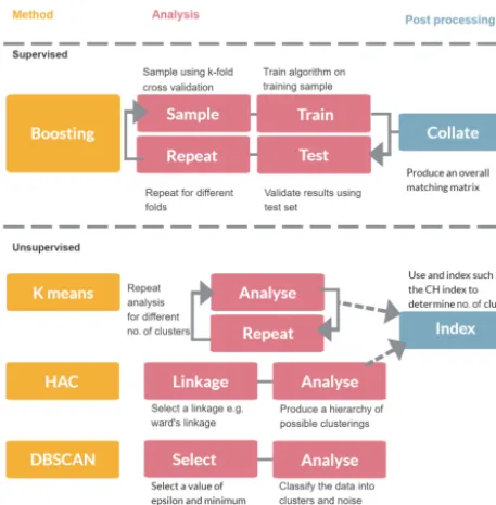
Figure 1.Overview of different analysis approaches.
generated aerosol or ambient data. See Sect. 2.3 for further details on data preparation for HAC.
Furthermore, data analysis using HAC can take a matter of hours, if not days, depending on the number of particles. The time requirements for HAC are betweenN2andN3 mean-ing that a doublmean-ing of the number of particles will require between 4 and 8 times as much time. Such time require-ments mean that not only is the method already quite slow, but will get increasingly slower as more data are collected, which may limit the real time effectiveness of the method.
Within the Python programming language, a package called Scikit-learn (Pedregosa et al., 2011) offers imple-mentations of several unsupervised methods. Some of these methods, i.e. Affinity Propagation, Mean-shift, Spectral Clustering and Gaussian mixtures are not explored as they will scale poorly as the number of particles increases (Pe-dregosa et al., 2011). Instead, our analysis is focused onk -means, HAC and DBSCAN which can be used on larger data-sets.
For HAC we continue to use the fastcluster package (de-scribed in Sect. 2.3). Sci-kit learn does have a HAC imple-mentation but it is not as fast or memory efficient. We do use sklearn for DBSCAN andk-means, although if one was to use DBSCAN for ambient data we would suggest explor-ing alternatives such as ELKI (Schubert et al., 2015) as the sci-kit learn implementation of DBSCAN by default is not memory efficient making it difficult to utilize for more than 30 000 particles. Sci-kit learn has a fast implementation for gradient boosting, so this is used.
Figure 2.Overview of preprocessing steps for WIBS data.
2 Methods
In this section we discuss the variety of approaches that could be used to classify particles such as bacteria, fungal spores or pollen. In Sect. 2.1 we provide an overview of the instrument used to collect the data. In Sect. 2.2 we discuss the variety of decisions that need to be made prior to passing the data to the machine learning algorithms which are discussed in Sect. 2.3–2.6. An overview of the different methods is given in Fig. 1.
2.1 Instrumentation
The Wideband Integrated Bioaerosol Sensor (WIBS) col-lects size, shape and fluorescence measurements (Kaye et al., 2005). The size is a single measurement; the shape measure-ment consists of four measuremeasure-ments (one for each quadrant) which are combined to produce a single asymmetry factor measurement. A more precise definition of asymmetry factor has been provided previously in the literature (Gabey et al., 2010).
To measure fluorescence, the particle is irradiated with UV light at 280 and 370 nm from the firing of two xenon sources. Fluorescence emission is collected via two collection chan-nels in the ranges 310–400 and 420–600 nm. The 370 nm xenon radiation lies within the first detection range and hence elastically scattered light from the particle, sufficient to satu-rate the detection amplifier, is received. This signal is there-fore discarded.
2.2 Data preparation
Prior to analysis using the machine learning algorithm we may choose to make a variety of decisions to pre-process the data with the aim to improve performance (see Fig. 2). An overview for the decisions often made are outlined below.
First we may elect to remove particles which are non-fluorescent. Forced trigger data are collected which is a mea-surement of the instrument response when particles are not present. We then set a threshold, for which if a particle fails to exceed this threshold in at least one of the fluorescent chan-nels we conclude that the particle is non-fluorescent. Usually we set the threshold to be three standard deviations above the average forced trigger measurement although a recent labo-ratory study has suggested that nine standard deviations may be more appropriate (Savage et al., 2017).
Another threshold is usually then applied to the size. A size threshold of 0.8 µm is usually applied as detection ef-ficiency of the instrument drops below 50 % at this point. (Gabey, 2011; Gabey et al., 2011; Healy et al., 2012b).
Natural logarithms of the size and the asymmetry factor are often taken as these measurements are often log normally distributed and it is postulated that this will increase perfor-mance in the case of hierarchical agglomerative clustering.
It is also widely regarded that standardizing the data prior to analysis is utmost importance (Milligan and Cooper, 1988). We often subtract the average measurement in each of the five variables and divide by the standard deviation, often referred to as “standardizing using thezscore”. Standardiza-tion is used to prevent variables with larger magnitude, such as the fluorescent measurements, from dominating the analy-sis. An alternative approach to standardizing is to divide each of the five variables by the range.
2.3 Hierarchical agglomerative clustering
In order for particles to be clustered, we need to define a mea-surement of how similar two clusters are. These similarity measures are often referred to as linkages. We use the Python package fastcluster (Müllner, 2013) which provides mod-ern implementations of single, complete, average, weighted, Ward, centroid and median linkages (Müllner, 2011). A thor-ough detailing of the definitions of the different linkages can be found in the fastcluster manual (Müllner, 2013). For the memory efficient mode, which is essential when using the al-gorithm for large data sets, only Ward, centroid, median and single linkages are available.
Initially each particle is placed into an individual cluster. Next, using the linkage selected, the two most similar clus-ters are merged. The merging process is repeated until all the particles are placed in a single cluster, which provides a clustering from k=1, . . . , N, where k is the number of clusters andN is the number of particles being analysed. A cluster validation index such as the Cali´nnski–Harabasz in-dex (Cali´nski and Harabasz, 1974) is then used to identify an
\
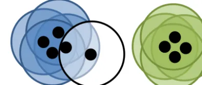
Figure 3.Visual representation of DBSCAN. Here each point is represented as a black dot and its neighbourhood is represented by a circle. Hereis the radius of the circle and the minimum number of points is 3. Four points have each been placed into the blue cluster and green cluster, all of which having at least 3 other points in their neighbourhood. One point is classified as noise as it has only 1 other point in its neighbourhood.
appropriate number of clusters. The index is maximized for clusterings that contain compact clusters that are far apart.
2.4 K-means clustering
K-Means clustering is designed to place particles into k clusters. However we can repeat the method multiple times, e.g. fork=1, 2, . . . , 10, wherekis the number of clusters. Similar to HAC we can then use a cluster validation index to determine which choice ofkgives the most effective results. The method works as follows. Initiallykcluster centroids are set by selectingk particles at random. The rest of the particles are then placed into thesek clusters depending on which of the centroids the particle is closest to. At this point a new centroid is calculated for each cluster. The process is then repeated many times until convergence occurs and the centroids do not change significantly from one iteration to the next.
2.5 DBSCAN
For DBSCAN we set two parameters, the radius for a neigh-bourhood, and the number of particles required for a neigh-bourhood to be identified as dense.
Initially a random point, say A, is selected. If there are suf-ficient number of points in the neighbourhood of A then all the points in A’s neighbourhood are also checked and so on, until the cluster has fully expanded and there are no points left to check. Should the point not have a sufficient number of other points in its neighbourhood then it is left unclassi-fied. Further points are then selected and the above process is repeated until all points have been considered.
Figure 4. Four example matching matrices. Immediately below each matrix is the percentage of particles placed into the same clus-ter for both clusclus-terings in each case. At the very bottom we have the adjusted rand score.
2.6 Gradient boosting
A basic decision tree is constructed by considering each pos-sible split across all variables and evaluating which split best divides the data. For example, we may consider the third flu-orescence channel and split the data on the basis of whether the measurement is more or less than 10 arbitrary units (AU). This process is then repeated many times until a tree is built. There are two ways in which trees can be combined into an ensemble. The first is by averaging multiple trees in the hope to produce a more accurate classification as is the case in random forests and bagging classifiers (Breiman, 2001, 1996). In the case of random forests and bagging, the data set is sampled with replacement, meaning that the same par-ticle could be selected more than once or not at all. Sampling in this way enables the algorithm to produce a subtly dif-ferent version of the data from which to build each tree. In addition, when using a random forest, instead of considering all possible variables to use to split the data, only a random subset is used.
Alternatively we can fit a single decision tree to the data, evaluate where the tree is performing well and then fit a sec-ond tree to the particles in the data for which the current model is performing poorly. This process can be repeated many times, each time adding a new tree to the model in the hope of making an improvement. This approach is known as AdaBoost (Freund and Schapire, 1997). Gradient boosting is an extension of AdaBoost to allow for other loss functions (Friedman, 2001).
For the current study we elect to use gradient boosting to indicate the performance of the supervised approach since it was the best performer for the Multiparameter Bioaerosol Spectrometer, a similar UV-LIF spectrometer similar to the WIBS but with single waveband fluorescence, 8 fluorescence detection channels and very high shape analysis capability (Ruske et al., 2017).
2.7 Evaluation criteria
To aid in evaluating how well methodologies performed we used two tools: the matching matrix (Ting, 2010) and the ad-justed rand score (Hubert and Arabie, 1985).
In Fig. 4 we present four different matching matrices. To produce these matrices we compared: two random cluster-ings with approximately 50 % of the data in each cluster (A); two random clusterings each with 80 % and 20 % of the data in each of the two clusters, respectively (B); two identical clusterings (C); and two clusterings which were nearly iden-tical except one data point had been placed into a third cluster for one of the clusterings.
2.7.1 Matching matrix
The matching matrix, often referred to as a confusion matrix, can be used as an aid in comparing two clusterings.
In the case of the current paper, we use this to compare the output from an algorithm with labels assigned to each particle. We may assign labels to indicate what broad type the particle is (e.g. 1 if the particle is bacteria, 2 if the particle is fungal etc.) or we may assign labels to indicate what sample a particle is from (e.g. 1 if the particle isBacillus atrophaeus, 2 if the particle isE. colietc.)
Consider example C in Fig. 4. This matching matrix com-pares two clusterings each containing two clusters. Each row corresponds to a cluster in the first clustering and each col-umn corresponds to a cluster in the second clustering. The el-ement in the first row and the first column (in this case 784) indicates the number of particles that were placed into the first cluster in the first clustering that were also placed into cluster 1 in the second clustering. Two identical clusterings will produce a matching matrix that has non-zero values only the diagonal.
A and B in Fig. 4 are examples of poor performance and C and D are examples of very good performance.
2.7.2 Adjusted Rand score
When evaluating a large number of clusterings, it may be useful to use a statistic to summarize the information in the matching matrix. In a previous study (Ruske et al., 2017), we used percentage of particles correctly classified as a statistic for indicating performance. This is an easy to interpret statis-tic, but can be misleading when used on imbalanced data. In both example A and B, we have two randomly generated clusterings. However in B we have 80 % of the data points placed into the first cluster, whereas in A the data points are approximately equally distributed between the two clusters. The percentage of points which are placed into the same clus-ter for both clusclus-terings are 52.2 % and 68.3 % for A and B, respectively. We can see that the more imbalanced a data set is, the more likely data points are to be placed into the same clusters. It is for this reason we elect to use an alternative statistic: the adjusted rand score. This statistic attains a value of approximately zero for both A and B.
the adjusted rand score. However our initial tests (not pre-sented), indicated that calculation of the mutual information often required an order of magnitude more time than the cal-culation of the adjusted rand. Therefore, we elected to use the adjusted rand score for the current study.
3 Data
The efficacy of the different data analysis approaches was evaluated using three different data sets. The first of which comprised several industry standard polystyrene latex spheres of various different sizes and colours. This data set was first analysed in Crawford et al. (2015), where hierarchi-cal agglomerative clustering was successfully applied to the data yielding a classification accuracy of 98.2 %. This data set presents a simple challenge for which we would expect any reasonable algorithm to be able to discriminate between the different sizes and colours of particles.
To further extend the previous analysis in Crawford et al. (2015) we include two data sets collected in 2008 and 2014 which are similar to data previously published using the Mul-tiparameter Bioaerosol Spectrometer (Ruske et al., 2017). A subsection of the data collected 2014 has previously been analysed in the Appendix of Crawford et al. (2017). These data sets consist of various different pollen, fungal, bacterial and non-biological samples, and should present a much more difficult challenge for the algorithms.
The samples of laboratory generated aerosol were col-lected as follows. Material was aerosolized into a large, clean HEPA filtered chamber, which incorporated a recirculation fan. TheBacillus atrophaeusandEscherichia coli (E. coli) bacteria were aerosolized into the chamber using a mini-nebulizer (e.g. Hudson RCI Micro-Mist mini-nebulizer) as were the salt and phosphate buffered saline samples. The dry sam-ples, which included the pollen, and fungal samples were aerosolized directly into the chamber from small quantities of powder utilizing a filtered compressed air jet. The diesel smoke and grass smoke samples were generated by burning a small amount within a fume cupboard using a smoker (a piece of bespoke equipment). The bacterial samples were ei-ther washed or unwashed and diluted or undiluted.
We present a summary of the number of particles for each sample after a fluorescent threshold of 3σ and 9σ is applied in Tables 1, 2 and 3. In 2008 the thresholds are constructed using forced trigger data collected at the same time as the experiment, whereas in 2014 the thresholds are constructed using forced trigger data collected using the same instrument at an earlier date. Ideally, the threshold for the data collected in 2014 would be constructed using forced trigger data col-lected at the same time as the laboratory data, but we can see in Fig. 8 that the threshold we have constructed is successful in removing the vast majority of NaCl samples collected.
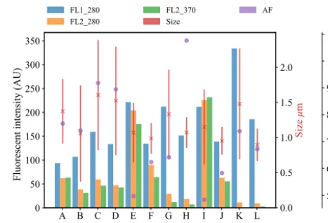
Plots of the average fluorescent characteristics and size and shape for each sample are provided in Figs. 5, 6 and 7
A B C D E F G H I J K L
Sample 0 50 100 150 200 250 300 350
Fluorescent intensity (AU)
0.0 0.5 1.0 1.5 2.0 S iz e m 5 6 7 8 9 10 11
Asymmetry factor (AU)
FL1_280 FL2_280
FL2_370 Size
AF
Figure 5.Average fluorescent characteristics for the bacterial sam-ples collected in 2008. The error bars in red indicate a range of±1σ
for each sample.
M N O P Q R S T U V W
Sample 200 400 600 800 1000 1200
Fluorescent intensity (AU)
0 2 4 6 8 10 12 S iz e m 6 8 10 12
Asymmetry factor (AU)
FL1_280 FL2_280
FL2_370 Size
AF
Figure 6. Average fluorescent characteristics for the remaining samples collected in 2008. The error bars in red indicate a range of±1σ for each sample.
after a fluorescent baseline of 3σ has been applied. Similar plots have been produced using a 9σ threshold and can be found in the repository released alongside the paper (see the “Code and data availability” section for further details). Plots and tables for the polystyrene spheres previously published in Crawford et al. (2015) are omitted.
Table 1.The number of particles remaining after a fluorescent threshold of 3σor 9σ was applied for each of the bacterial samples collected in 2008. Each sample was either washed or unwashed and diluted or undiluted. Each sample was either washed or unwashed, and diluted or undiluted as indicated by a check mark in the corresponding column.
ID Sample W Dil. n >3σ n >9σ
A Bacillus atrophaeusspores 952 34
B X 52 4
C X 1171 217
D X X 241 38
E Bacillus atrophaeusvegetative cells 4779 1915
F X 1488 264
G X 1884 573
H X X 2064 194
I E. coli. 3684 1547
J X 1448 371
K X 2365 1461
L X X 835 302
Table 2. The number of particles remaining after a fluorescent threshold was applied for each of the non-bacterial samples col-lected in 2008.
ID Sample Category n >3σ n >9σ
M Bermuda grass smut Fungal 2681 423
N Johnson grass smut I Fungal 1209 259
O Johnson grass smut II Fungal 2673 378
P Birch pollen Pollen 111 56
Q Paper mulberry pollen I Pollen 233 209
R Paper mulberry pollen II Pollen 397 103
S Ragweed pollen I Pollen 123 34
T Ragweed pollen II Pollen 209 117
U Diesel smoke Interferent 11 5
V Grass smoke I Interferent 2542 231
W Grass smoke II Interferent 815 68
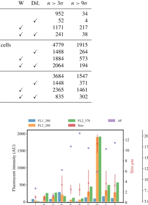
The data collected is using a WIBS version 3 which is lim-ited to a detection range of approximately 0.5–12 µm, which limits the ability of the instrument to detect intact pollen grains. The vast majority of the equivalent optical diame-ters (EODs) for the pollen samples collected are much lower than the measurements for intact pollen grains and are there-fore likely to be pollen fragments, as was the case in Her-nandez et al. (2016). The exception is the paper mulberry samples where there are differences across each of the sam-ples. In 2008, sample Q which shows a size range similar to the other pollen samples is most likely to consist entirely of pollen fragments, whereas sample R shows a much wider size range which is likely to comprise of both fragmented and intact pollen. The collection of both fragmented and intact pollen has previously been shown to occur in Savage et al. (2017). In 2014, for sample H, the size range is much larger, consistent with the hypothesis of measuring intact pollen.
A B C D E F G H I J
Sample 0 500 1000 1500 2000
Fluorescent intensity (AU)
0 2 4 6 8 10 12 S iz e m 5.0 7.5 10.0 12.5 15.0 17.5 20.0
Asymmetry factor (AU)
FL1_280 FL2_280
FL2_370 Size
AF
Figure 7. Average fluorescent characteristics for the different aerosol samples collected in 2014. The error bars in red indicate a range of±1σfor each sample.
Paper mulberry has been previously been sampled in Healy et al. (2012a), using a WIBS version 4 in a low-gain mode which allows for the collection of particles up to approxi-mately 31 µm. In this study, the size range of the paper mul-berry was 13.6±6.2, indicating that if sample H is intact pollen we may only be measuring part of the distribution.
Table 3.The number of particles remaining after a fluorescent threshold was applied to each of the samples collected in 2014. Whether a bacterial sample was washed or unwashed is specified after the sample name.
ID Sample Category n >3σ n >9σ
A Bacillus atrophaeusspores (unwashed) Bacteria 1728 684
B Bacillus atrophaeusspores (washed) Bacteria 1322 608
C E. coli(unwashed) Bacteria 1290 632
D Puffball spores I Fungal 504 248
E Puffball spores II Fungal 35 3
F Puffball spores III Fungal 16 1
G Aspen pollen Pollen 74 31
H Paper mulberry pollen Pollen 541 537
I Poplar pollen Pollen 104 50
J Ryegrass pollen Pollen 21 15
K Fuller’s earth Interferent 61 20
L NaCl Interferent 3 0
M Phosphate buffered saline Interferent 35 3
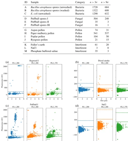
Figure 8.Scatter plots of fluorescence vs. size for four of the samples. Two of the samples were collected in 2008(a, b)and two were collected in 2014(c, d); two are biological(a, c)and two are non-biological(b, d).
4 Results
In Sect. 4.1, 4.2, 4.3 we present the results using HAC, DB-SCAN and gradient boosting, respectively. A summary of the findings for each method and an indication of how the num-ber of clusters are determined are shown in Table 4.
4.1 Hierarchical agglomerative clustering
dif-Table 4.Summary of findings and considerations for method selection.
Method Summary No. of clusters
HAC – Does not rely on training data.
– The conclusion we make when using the CH index may be incorrect when a large proportion of the particles are from one broad class.
– How the data were prepared greatly impacted upon per-formance.
– Particles from different categories were sometimes clus-tered together, e.g. pollen with fungal.
Determined using the maximum value of the CH index produced for clusterings containing
between 1 and 10
clusters.
DBSCAN – Produced a clustering which contained three distinct clusters each containing primarily one broad class of bioaerosol in the case of one of the data sets.
– Data preparation greatly impacted upon performance.
– It is not clear at this point whether the values of epsilon and the minimum number of points would be applicable to ambient data.
Naturally determined by setting epsilon and the minimum number of points required for a neighbourhood.
Gradient boosting
– Performance was consistently good irregardless of data preparation provided that a threshold, either 3 or 9 stan-dard deviations, was applied to the fluorescence measure-ments
– Relies on adequate training data being collected and it is not clear at this point whether the data collected will be sufficient.
Always the same as the number of groups in the training data.
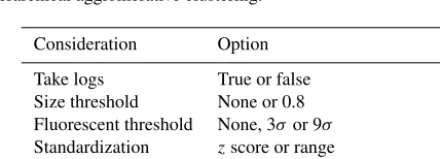
ferent approaches to prepare the data which are shown in Table 5. Following this, 96 possible combinations of these considerations were applied to the data and the hierarchical agglomerative clustering routine was used to cluster the re-sultant data in each case. For each of the 96 hierarchies pro-duced, the clusterings containing between 1 and 10 clusters were extracted. Subsequently, a value of the adjusted rand score comparing each of these 10 clusterings to the known la-bels was calculated. These values of the adjusted rand score would be unavailable during an ambient campaign but are used here to measure the similarity of each clustering to the known labels in order to indicate overall performance and highlight which of the first 10 clusterings was most similar to the known labels. Values of the Cali´nnski–Harabasz index (CH index), an index which is usually used in an ambient campaign to determine the number of clusters, were also cal-culated. The number of clusters in the clustering for which the maximum value of the CH index was attained can then be compared to the clustering which is most similar to the known labels to determine if the CH index attains a maxi-mum for the clustering which is most similar to the known labels.
Table 5.Outline of the different approaches tested when using hi-erarchical agglomerative clustering.
Consideration Option
Take logs True or false
Size threshold None or 0.8
Fluorescent threshold None, 3σor 9σ
Standardization zscore or range
Linkage Ward, centroid, median or single
4.1.1 Impact of data preparation
In the case of the PSL data set, we see that HAC has pro-duced a clustering with 5 clusters which is very similar to the known labels. The best performance occurred when us-ing a fluorescent threshold of 9 standard deviations, albeit 3 standard deviations produced a similarly high value of the adjusted rand score (0.958).
The maximum adjusted rand scores attained for the labora-tory generate aerosol collected in 2008 and 2014 were 0.567 and 0.747. Lower scores are to be expected since we would anticipate laboratory generated aerosol to be more complex than polystyrene latex spheres and hence more difficult to discriminate. The adjusted rand score of the best data strategy of the 96 tested, as indicated by the height of the green bar, is larger than the corresponding adjusted rand score for the strategy suggested in Crawford et al. (2015), indicating that potentially a different strategy may yield better results. How-ever, the best performing strategy was not consistent across both the 2008 and 2014 data.
In particular, the best strategy in 2008 was found to be tak-ing logs; ustak-ing a size threshold of 0.8 µm; ustak-ing a fluorescent threshold of 3 standard deviations; standardizing using the range and using Ward linkage. In 2014, the highest value of the adjusted rand score was obtained by not taking logs, not applying a size threshold, using a fluorescent threshold of 9 standard deviations and using the centroid linkage. Since our findings are inconsistent across the two laboratory gener-ated aerosol data sets it becomes difficult to provide a better recommendation for data preparation other than the strategy suggested in Crawford et al. (2015).
In addition, there was a substantial difference between the quality of results attained when using a fluorescent threshold of 3 or 9 standard deviations. In 2008, we see a decrease in the adjusted rand score from 0.482 to 0.277 when using 3 and 9σ, respectively. In 2014, we see an increase in the adjusted rand score from 0.462 to 0.625 when using 3 and 9σ, respectively.
It is possible that the difference in performance when using the different thresholds could be in part explained by the fluo-rescent threshold in 2014 being constructed using forced trig-ger data collected at a different time to the laboratory data, or by the fluorescence properties differing across the two data sets. But this differing behaviour when using different data preparation does need to be investigated further with addi-tional laboratory data sets and in the context of ambient data. Nonetheless, the differing conclusions across the two data sets as to which data preparation is preferable does highlight the importance of repeating data collection and demonstrat-ing conclusions are consistent across multiple experiments.
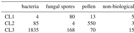
The adjusted rand score is often quite difficult to interpret, so we provide matching matrices for the best and worst case scenario using the current data preparation strategy in Ta-bles 6 and 7. In the best case scenario we are able to dis-criminate between the pollen and the rest of the data placing 86.8 % of the pollen into Cluster 2. Most of the bacteria is also placed into Cluster 3 with 66.6 % of the fungal spores.
Figure 9.Performance of hierarchical agglomerative clustering us-ing the adjusted rand score for the data sets tested across differ-ent data preparation strategies. The number of clusters concluded in each case is indicated at the bottom of each bar.
A third of the fungal spores are differentiated from the rest of the data and placed into Cluster 1. In the worst case scenario two clusters are provided both primarily containing bacteria. In this case we can conclude that algorithm has failed to dif-ferentiate between any of the biological classes, in part due to the CH index concluding there are 2 clusters.
4.1.2 Impact of the Cali ´nnski–Harabasz index
At the base of each bar in Fig. 9 we provided the number of clusters in the clustering for which the adjusted rand score presented was obtained. For the darker bars, this number rep-resents the number of clusters in the clustering for which the highest value of the adjusted rand score was obtained across the clusterings containing between 1 and 10 clusters. For the lighter bars, this number represents the number of the clus-ters in the clustering for which a maximum of the CH index was attained.
in-dex has attained a maximum at 4 clusters instead of 5 is not concerning, since concluding 4 clusters instead of 5 has very little impact upon performance.
The final case is in 2008, using a fluorescent threshold of 9 standard deviations. Here the clustering which is most simi-lar to the known labels is the clustering containing 5 clusters, whereas the CH index attains a maximum for the clustering containing only 2 clusters. The 2 cluster solution in this case is very dissimilar from the known labels.
In the cases where a maximum for the CH index was at-tained for a clustering containing 2 clusters, i.e. in 2008 using 9σ and in 2014 using 3σ, 78.6 % and 76.5 % of the particles were from a bacterial sample. Conversely in 2008 using 3σ and in 2014 using 9σ, 65.4 % and 68.4 % of the particles analysed were bacteria.
To investigate the possibility of a relationship between the proportion of the data which is contained in the category con-taining the largest number of particles and the tendency of the CH index to conclude that there are 2 clusters we produced data simulated from 3 normal distributions in 3 dimensions. Each of the clusters was centred around [0, 0, 0], [5, 5, 5], [10, 10, 10] and the co-variance matrix was set toσI3, where I3 is the 3 by 3 identity matrix. The value ofσ was varied from 1 to 3 to produce a range of variation in the simula-tions. We elected to produce this simulated data from nor-mal distributions rather than the laboratory data collected to remove any potential confounding issues such as the fluo-rescent threshold used. The proportion of the data that was contained in the dominant cluster was varied from 50 % to 99 %. Each simulation was repeated 100 times to provide an indication of the frequency the CH index attains a maximum for the 3 cluster solution.
In Fig. 10 we see that there is a point where the frequency for which the CH index attains a maximum for the cluster-ing containcluster-ing 3 clusters starts to decrease. The proportion of data points that needs to be placed in the dominant cluster before this decrease in performance of the CH index is seen decreases as the variability in the data increases.
This incorrect conclusion when using the CH index when analysing data for which a large proportion of data are of one particular type is problematic when analysing biological aerosol, since we may expect the quantity of bacteria to be an order of magnitude greater than the fungal spores, and for the quantity of fungal spores to be an order of magnitude greater than the pollen (Després et al., 2012; Gabey, 2011). In future studies it may therefore be necessary to explore the use of other indices for determining the number of clusters.
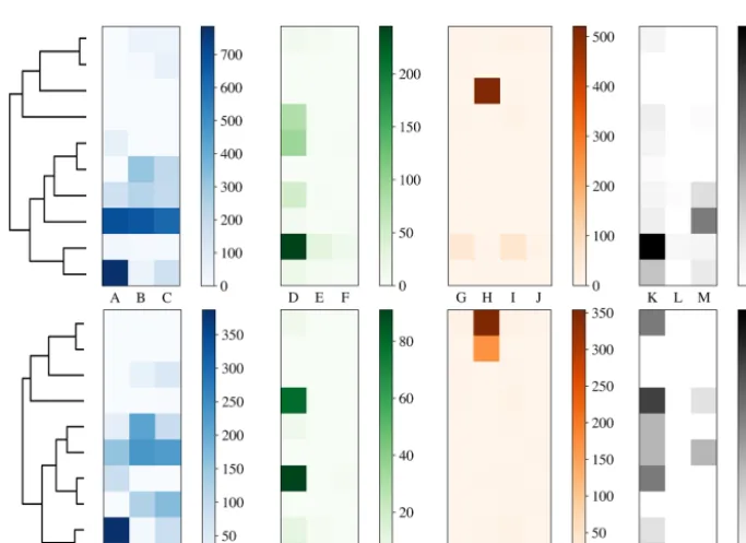
4.1.3 Breakdown of the hierarchies
To more clearly understand how data have been clustered us-ing HAC we have presented dendrograms for the laboratory data collected in 2008 and 2014 in Figs. 11 and 12 alongside heat maps of the matching matrices to indicate the cluster composition of the 10 cluster solution broken down by
sam-Figure 10.Percentage of simulations for which the CH index at-tained a maximum for the clustering containing 3 clusters against the proportion of the data which is placed into a dominant cluster.
ple. The hierarchy produced using the strategy suggested in Crawford et al. (2015) is presented at the top of each plot whereas a modification of this strategy using a threshold of 9 standard deviations as suggested by Savage et al. (2017) is presented at the bottom.
Each row of the heat map corresponds to a particular clus-ter and each column corresponds to a particular sample. The intensity of each box corresponds to the quantity of parti-cles placed into a particular cluster from a particular sam-ple. Bacterial, fungal, pollen and non-biological samples are grouped together in blue, green, orange and black, respec-tively. Different scales are used for the different groups to prevent the dominant class from obscuring information in the other classes.
In 2008, the majority of the bacteria is placed into a sin-gle cluster for both 3σ and 9σ. The fungal and a number of pollen particles are placed into the same two clusters when using 3σ and into one cluster when using 9σ. The non-biological samples, consisting primarily of grass smoke, are clustered mostly with bacterial samples, possibly due to their similar size. In addition, there are two clusters when using 3σ and three clusters when using 9σ containing primarily pollen.
In 2014, pollen has been placed primarily into 1 or 2 clus-ters. Some of the fungal samples have been placed into a singleton cluster. For both thresholds the bacteria is grouped with some of the fungal samples. The non-biological mate-rial has almost entirely been removed by the threshold and the remaining material has been divided among a number of the clusters.
Table 6.Matching matrix for the best case scenario when using the current data preparation strategy with 9σ on the data collected in 2014.
bacteria fungal spores pollen non-biological
CL1 4 80 13 5
CL2 85 4 550 3
CL3 1835 168 70 15
Table 7.Matching matrix for the worst case scenario when using the current data preparation strategy with 9σ on the data collected in 2008.
bacteria fungal spores pollen non-biological
CL1 547 69 298 0
CL2 6373 991 221 304
the paper mulberry sample, whereas in 2008 the fungal and pollen material may be grouped due to presence of a larger number of pollen fragments. It is therefore important when interpreting results from an ambient campaign that it is possi-ble that clusters may contain more than one broad biological class.
Also note that this potentially undesirable grouping of ma-terial from two different classes has occurred prior to the final stages of the algorithm and therefore will be apparent in the final solution regardless of the number of clusters concluded, and cannot be rectified by using a different validation index.
4.2 DBSCAN
One of the main difficulties of using DBSCAN is selecting the minimum number of points to form a neighbourhood and the radius of the neighbourhood (Khan et al., 2014). For 3σ and 9σ usingzscore standardization, taking logs of the size and asymmetry factor and removing particles smaller than 0.8 µm we repeat the DBSCAN algorithm for a variety of (neighbourhood radii) and minimum number of points val-ues. The range of values ofwe test is 0.1, 0.2, . . . , 1.0. The range of minimum number of points is set using the follow-ing range relative to the number of particles collected 0.1 %, 0.2 %, . . . , 1.0 %, 2.0 %, . . . , 10.0 %.
We found wide variety of performance across the differ-ent parameters. Often high accuracy could be obtained when using a high value of the minimum number of points but this resulted in removing a substantial portion of the data. In Fig. 13 we filter our results using a range of thresholds for the maximum number of points that can be left unclas-sified (5 %, 10 %, . . . 60 %) and plot the corresponding best performance under this filter. In all the data sets there was a point of diminishing returns where no further benefit could be attained by removing any more of the data. In the case of the PSL data, this point happened after removing around 5 %
Table 8.Matching matrix for the best case scenario when using DBSCAN with 9σ,=0.4 and a minimum number of points of 0.7 % on the 2014 data.
bacteria fungal pollen non-biological
Unclassified 329 169 134 16
CL1 0 0 490 0
CL2 12 80 4 0
CL3 1583 3 5 7
of the particles. For the laboratory data sets between 25 % and 40 % of the data were left unclassified before a peak in performance was attained. Nonetheless, we note in the case of the laboratory data collected in 2014 and using a 9σ flu-orescent threshold, we can attain performance similar to that which we attain for the PSL data.
In order to investigate further a choice ofand the mini-mum number of points which would maximize performance in terms of the adjusted rand score we plot the adjusted rand score for each test across all of the data sets. In Fig. 14 we see that there is a large window of different values for which a higher value of the adjusted rand score can be achieved on the PSLs. Contrary to this, in 2008 when using 9σ there is a very narrow window for which higher values of the adjusted rand score could be attained. It can also be seen that as increases the number of points required to create a cluster needs to be increased to compensate.
Overall our results indicate setting =0.3 and =0.4 when using 3σ and 9σ, respectively. The best results can then be obtained by setting the number of points between 0.4 % and 0.7 % of the data when using an of 0.3 % and 0.7 % and 1.0 % when using anof 0.4. However, future re-search will be required to demonstrate these conclusions are applicable when studying ambient data.
Figure 11.Dendrogram truncated at 10 clusters (left) for laboratory data collected in 2008 alongside a heat map of matching matrix (right) indicating cluster composition by each sample segregated by bacteria, fungal, pollen and non-biological in blue, green, orange and black, respectively. Separate scales are used for each broad class to prevent dominant class obscuring detail in the other classes. Hierarchies for 3σ
(top) and 9σ(bottom) are presented.
Figure 12.Dendrogram truncated at 10 clusters (left) for laboratory data collected in 2014 alongside a heat map of matching matrix (right) indicating cluster composition by each sample segregated by bacteria, fungal, pollen and non-biological in blue, green orange and black, respectively. Separate scales are used for each broad class to prevent the dominant class obscuring detail in the other classes. Hierarchies for 3σ (top) and 9σ(bottom) are presented.
4.3 Gradient boosting
We conducted a similar analysis varying data preparation ap-proaches as in Sect. 4.1. We found data preparation to have a very small impact upon performance when using gradient boosting as long as some kind of fluorescence threshold is applied where a high value of the adjusted rand score was
obtained regardless of whether we took logs, what standard-ization was used or the size threshold imposed.
10 20 30 40 50 Percentage of data unclassified 0.0 0.2 0.4 0.6 0.8 1.0
Adjusted rand score PSL 3
2008 3 2014 3
PSL 9 2008 9 2014 9
Figure 13. Adjusted rand score using different thresholds of per-centage of points we allow to be left in the analysis for DBSCAN.
0.2 0.4 0.6 0.8 1.0 0.2 0.4 0.6 0.8 1.0
0.1 0.5 0.9 1.0 5.0 Points (%) 0.2 0.4 0.6 0.8 1.0
0.1 0.5 0.9 1.0 5.0 Points (%) 0.0 0.2 0.4 0.6 0.8 1.0
Figure 14.Adjusted rand score for DBSCAN, over a range differ-ent values ofand minimum number of points required to form a neighbourhood. The minimum number of points is expressed rela-tive to the total number of points. The columns correspond to 3 and 9σ, respectively. The rows correspond to the PSL, 2008 and 2014 data, respectively.
the previous sections we provide matching matrices of the worst case scenario and best case scenario when using gradi-ent boosting using the currgradi-ent data preparation in Tables 10 and 11. In the best case scenario we provide a very good clas-sification with very small errors (AR=0.933).
In the worst case scenario a similar performance is achieved (AR=0.882). Nonetheless, a few particles are incorrectly classified within the fungal spore and pollen classes. The classification for the bacteria is still very strong and most of the remaining non-biological particles are cor-rectly classified. The non-biological samples have been re-moved from this data set prior to gradient boosting being ap-plied when using a fluorescent threshold of either 3σ or 9σ. We elect to remove these particles since too few of the non-biological samples that exceed either threshold to produce a viable training class.
Table 9.Matching matrix for the worst case scenario when using DBSCAN with 3σ,=0.3 and a minimum number of points of 0.4 % on the 2008 data.
bacteria fungal pollen non-biological
Unclassified 5858 1893 636 752
CL1 15 025 15 44 2616
CL2 80 4655 393 0
Figure 15.Performance of gradient boosting for the different data sets when using 3σand 9σ.
4.4 K-means
Similar to the findings presented in Ruske et al. (2017),k -means performed poorly and hence the results are omitted from the main text. The results are available in the reposi-tory published alongside the paper (see the “Code and data availability” section for further details).
5 Conclusions
We evaluated a variety of different methods that could be used for classification of biological aerosol. Gradient boost-ing offered the best performance consistently across the dif-ferent data preparation strategies and the difdif-ferent data sets tested. That being said it is unclear at this point how this will translate to ambient data and whether or not the training data currently collected will be sufficient to outline the variety of environments that could potentially be studied.
Should there not be sufficient training data available an unsupervised approach may be required. In this case, a pos-sible alternative to HAC is provided. In the best case sce-nario DBSCAN, despite leaving a decent proportion of the data unclassified, was able to produce three distinct clusters containing predominantly one biological class each.
Table 10.Matching matrix for the best case scenario when using gradient boosting. This is when using 9σ on the 2014 data.
bacteria fungal pollen
bacteria 1911 8 19
fungal 7 219 29
pollen 6 25 595
Table 11.Matching matrix for the worst case scenario when using gradient boosting. This is when using 9σ on 2008 data.
bacteria fungal pollen non-biological
bacteria 6852 85 76 8
fungal 56 898 147 2
pollen 8 72 293 0
non-biological 4 5 3 294
we have provided details of what we believe to be sensible selections of epsilon and the minimum number of points on the basis of the laboratory data collected. However, it is un-clear at this point how effective these selections will be when analysing ambient data.
When applied the laboratory generated aerosol tested, we found that performance of HAC was in general much lower than what was achieved previously using the PSLs (Craw-ford et al., 2015). Performance was heavily dependent on the data preparation strategy used, and often results could vary substantially between different strategies and data sets, po-tentially due to differences in the fluorescence measurements across the two data sets. A potential issue with the CH index is highlighted, whereby we see a failure of the index to deter-mine the correct number of clusters as the size of the dom-inant class and variation in the data increases. Some of the pollen samples were clustered with the fungal samples when analysing the data from 2008. A number of the pollen parti-cles may be fragmented which may explain why this group-ing may occur. Similarly grass smoke was grouped with the bacterial samples, potentially due to their similar size. Cau-tion will therefore be required when applying the HAC algo-rithm to ambient data, and it must be noted in particular that material from two different classes may be placed into the same cluster and that the CH index may indicate an incorrect number of clusters if the data collected contains a significant quantity of one particular type of particle.
In the future, more laboratory generated aerosol particles will need to be collected to continue to evaluate the perfor-mance of the algorithms which we use. In addition, when gradient boosting was used we failed to classify the some of the pollen and fungal spore samples analysed. It is therefore possible that higher spectral instruments such as the spec-tral intensity bioaerosol sensor (Nasir et al., 2018), will be required to provide a more accurate classification.
Code and data availability. Part of the code used produce the
above paper is part of an ongoing development of a software suite for analysis of various UV-LIF instruments, available at https: //github.com/simonruske/UVLIF, last access: 5 November 2018, upon publication, and Ruske (2018a). Other code not currently in-cluded within the software package, i.e. code files which are used to produce the plots and figures specific to the current paper are avail-able at https://github.com/simonruske/AMT-2018-126, last access: 13 November 2018, and Ruske (2018b).
Appendix A: Comparison of particle size with other studies
Table A1.Average particle sizes for the current study compared with other studies. The sizes presented here are collated from the following studies [1] Healy et al. (2012a), [2] Savage et al. (2017), [3] Hernandez et al. (2016), [4] Pierucci (1978), [5] Carrera et al. (2007), [6] Crotzer and Levetin (1996), [7] Geiser et al. (2000), [8] Pinnick et al. (1995), [9] Fumanal et al. (2007), [10] Mäkelä (1996), [11] Kang et al. (2007), [2008] and [2014] are taken from the current study.
Sample Measurement type Size (µm) Reference
Paper mulberry pollen WIBS4 low-gain 13.6±6.2 [1]
WIBS3 7.18±4.74 [2008]
WIBS3 3.41±1.43 [2008]
WIBS3 11.27±1.74 [2014]
Miscroscopy 13.8 [11]
Ragweed pollen WIBS4 low-gain 24.5±7.6 [1]
WIBS3 3.51±1.38 [2008]
WIBS3 4.70±1.71 [2008]
Microscopy 13.02±0.12–14.86±0.16 [9]
Birch pollen WIBS4 low-gain 19.0±9.2 [1]
Betula lenta,nigraandpopulifoliapollen WIBS4 2.5±4.2 [3]
Birch pollen WIBS3 3.98±1.59 [2008]
Betula pollen (various) Microscopy 17.31±0.08–24.36±1.59 [10]
White poplar WIBS4A 18.7±1.9 [2]
White poplar fragments WIBS4A 7.4±4.0 [2]
Aspen pollen WIBS3 3.72±2.49 [2014]
Poplar pollen WIBS3 3.63±2.39 [2014]
Bermuda grass smut WIBS4 high-gain 4.7±2.2 [1]
WIBS3 3.57±1.16 [2008]
Microscopy 6.7×6.5 [6]
Johnson grass smut WIBS4 high-gain 8.9±1.5 [1]
WIBS3 3.47±1.00 [2008]
WIBS3 3.35±0.78 [2008]
Microscopy 13.9×12.6 [6]
Puffball spores Microscopy 3.5±0.24 [7]
WIBS3 2.50±0.85 [2008]
WIBS3 2.45±1.16 [2008]
WIBS3 3.39±1.76 [2008]
Fluorescence particle counter 2-4 [8]
Bacillus atrophaeusspores WIBS4A 2.2±0.4 [2]
WIBS3 1.00±0.40–1.60±0.78 [2008, 2014]
Microscopy 1.22±0.12 (length)
0.65±0.05 (diameter) [5]
Bacillus atrophaeusvegetative cells WIBS3 1.06±0.68–1.60±0.78 [2008]
E. coli WIBS4A 1.2±0.3 [2]
WIBS4 0.9±0.4 [3]
WIBS3 0.89±0.23–1.48±0.79 [2008, 2014]
Microscopy 1.67–3.08 (length)
Appendix B: ABC counts and average particle sizes To aid in comparing the data presented with other studies, we have presented Tables B1 and B2 which are very similar to the table in the appendices of Hernandez et al. (2016). A, B and C are used to denote particles which exceed the fluores-cent threshold in FL1_280, FL2_280, FL2_370, respectively. For example A is used to denote a particle that was only flu-orescent in the FL1_280 channel only. Combinations such as AB, AC, BC and ABC are used to denote particles which ex-ceed a fluorescent threshold in more than one channel. For example, AB is used to denote a particle that exceeded the fluorescent in both the FL1_280 and FL2_280 channels.
Table B1.For the data collected in 2008, a summary of size and fluorescent measurements for each sample to include: the number of particles in the sample (total), average equivalent optical diameter (EOD), standard deviation of the size (σ), the number of points that exceeded a fluorescent threshold of 3 standard deviations above the average forced trigger measurement (n >3σ), and ABC counts using a 3σthreshold.
n EOD σ n >3σ A B AB C AC BC ABC
Bacteria
Bacillus atrophaeusspores (unwashed) 5778 1.4 0.5 1015 322 200 74 113 48 90 168 Bacillus atrophaeusspores (unwashed, diluted) 1525 1.1 0.7 82 65 6 3 4 0 3 1 Bacillus atrophaeusspores (washed) 4694 1.6 0.8 1246 728 107 191 18 29 5 168 Bacillus atrophaeusspores (washed, diluted) 1786 1.5 0.8 280 183 21 30 9 10 12 15 Bacillus atrophaeusvegetative cells (unwashed) 6142 1.1 0.4 5546 409 693 771 75 79 287 3232 Bacillus atrophaeusvegetative cells (unwashed, diluted) 2192 1 0.2 1739 484 279 326 30 26 67 527 Bacillus atrophaeusvegetative cells (washed) 6002 1.3 0.6 1961 1797 3 139 0 1 1 20 Bacillus atrophaeusvegetative cells (washed, diluted) 2827 1.1 0.2 2218 2178 3 36 0 0 1 0 E. coli(unwashed) 4956 1.2 0.5 4097 366 578 174 179 69 868 1863 E. coli(unwashed, diluted) 2508 1 0.2 1778 751 309 82 99 27 263 247 E. coli(washed) 5669 1.5 0.8 2627 2508 1 99 0 0 0 19 E. coli(washed, diluted) 2104 0.9 0.2 1390 1383 0 5 0 0 2 0
Fungal
Bermuda grass smut 5220 3.6 1.2 2681 1446 7 34 271 495 81 347
Johnson grass smut I 2157 3.5 1 1211 76 3 3 796 128 92 113
Johnson grass smut II 5091 3.3 0.8 2675 217 8 1 1939 270 132 108
Pollen
Birch pollen 164 4 1.6 112 16 1 0 29 7 8 51
Paper mulberry pollen I 295 7.2 4.7 237 16 2 9 2 0 21 187
Paper mulberry pollen II 735 3.4 1.4 405 159 2 9 72 59 37 67
Ragweed pollen I 241 3.5 1.4 127 24 1 0 57 12 7 26
Ragweed pollen II 328 4.7 1.7 209 21 0 1 41 16 15 115
Non-biological
Diesel smoke 7900 1.1 0.4 16 3 4 0 5 0 0 4
Grass smoke I 9212 1.1 0.4 2976 1 234 0 2004 0 737 0
Table B2.For the data collected in 2014, a summary of size and fluorescent measurements for each sample to include: the number of particles in the sample (total), average equivalent optical diameter (EOD), standard deviation of the size (σ), the number of points that exceeded a fluorescent threshold of 3 standard deviations above the average forced trigger measurement (n >3σ), and ABC counts using a 3σthreshold.
n EOD σ n >3σ A B AB C AC BC ABC Bacteria
Bacillus atrophaeusspores (washed) 3321 1 0.4 2685 2545 1 15 1 81 1 41
Bacillus atrophaeusspores (unwashed) 2896 1 0.5 2248 85 15 2 1166 88 350 542
E. coli(unwashed) 2534 1.2 0.6 1640 268 10 5 439 239 48 631
Fungal
Puffball spores I 1739 2.5 0.8 35 3 1 0 27 1 3 0
Puffball spores II 553 2.5 1.2 16 2 0 0 12 1 0 1
Puffball spores III 1627 3.4 1.8 506 79 4 73 168 7 68 107
Pollen
Aspen pollen 398 3.7 2.5 74 5 1 0 35 1 11 21
Poplar pollen 375 3.6 2.4 104 7 0 3 45 4 21 24
Paper mulberry pollen 565 11.3 1.7 543 3 0 1 4 0 35 500
Ryegrass pollen 47 3.3 2.1 21 0 0 0 6 0 7 8
Non-biological
Fuller’s earth 3064 3.6 2.8 62 40 1 0 8 4 3 6
Phosphate buffered saline 3226 1.2 1.6 50 29 7 0 11 1 0 2
Table B3.Summary of properties for samples collected from 2008 and 2014, respectively, using a fluorescent threshold of 9σ.
2008
EOD σ n >9σ A B AB C AC BC ABC Bacteria
Bacillus atrophaeusspores (unwashed) 2.2 0.6 34 9 2 3 13 1 3 3
Bacillus atrophaeusspores (unwashed, diluted) 2.7 1.8 4 1 0 0 0 0 2 1
Bacillus atrophaeusspores (washed) 2.6 1.1 217 182 0 9 0 5 0 21
Bacillus atrophaeusspores (washed, diluted) 2.6 1 38 28 0 1 1 0 6 2
Bacillus atrophaeusvegetative cells (unwashed) 1.3 0.6 2051 273 326 132 33 19 184 1084
Bacillus atrophaeusvegetative cells (unwashed, diluted) 1.2 0.3 278 121 72 24 2 2 14 43
Bacillus atrophaeusvegetative cells (washed) 1.7 0.9 581 567 0 13 0 0 0 1
Bacillus atrophaeusvegetative cells (washed, diluted) 1.3 0.3 196 196 0 0 0 0 0 0
E. coli(unwashed) 1.5 0.7 1676 343 97 23 92 30 334 757
E. coli(unwashed, diluted) 1.1 0.2 413 333 23 4 12 4 17 20
E. coli(washed) 1.7 0.9 1516 1506 2 7 0 0 0 1
E. coli(washed, diluted) 1.1 0.3 349 348 0 0 0 0 1 0
Fungal
Bermuda grass smut 4 1.5 423 118 10 14 133 19 37 92
Johnson grass smut 4.2 1.3 259 0 0 1 171 0 29 58
Johnson grass smut II 3.8 1 378 2 2 0 340 0 29 5
Pollen
Birch pollen 4.5 1.8 57 7 0 0 9 0 2 39
Paper mulberry pollen I 7.8 4.6 212 22 0 7 3 0 30 150
Paper mulberry pollen II 3.9 2.1 107 17 2 2 21 0 39 26
Ragweed pollen I 4.7 1.4 34 0 0 0 11 0 2 21
Ragweed pollen II 5.5 1.5 117 2 0 0 9 0 10 96
Non-biological
Diesel smoke 1.1 0.2 6 0 3 1 1 0 0 1
Grass smoke I 2 0.5 236 0 1 0 218 0 17 0
Grass smoke II 2 0.4 68 0 0 0 64 0 4 0
2014
Bacteria
Bacillus atrophaeus(washed) 1.3 0.5 735 721 0 0 0 12 1 1
Bacillus atrophaeus(unwashed) 1.5 0.5 679 2 0 0 262 7 264 144
E. coli(unwashed) 1.6 0.7 669 55 0 0 209 135 13 257
Fungal
Puffball spores I 2.4 0.7 1 0 0 0 0 0 0 1
Puffball spores II 2 0 3 0 0 0 2 0 1 0
Puffball spores III 4.2 1.8 249 98 0 4 46 1 18 82
Pollen
Aspen pollen 5 3.2 31 1 0 0 10 2 7 11
Poplar pollen 4.4 2.9 50 3 0 0 14 1 19 13
Paper mulberry pollen 11.4 1.4 537 3 0 0 7 0 285 242
Ryegrass pollen 3.6 2.4 15 0 0 0 6 0 3 6
Non-biological
Fuller’s earth 4.5 3.2 20 9 0 0 4 1 3 3
Phosphate buffered saline 4.6 5.1 3 2 0 0 0 0 0 1
Appendix C: Summary of average properties of the different data sets
Table C1.Summary of particle measurements for the 2008 data set using a fluorescent threshold of 3σ.
Sample n >3σ FL1_280 FL2_280 FL2_370 Size AF
Bacillus atrophaeusspores (unwashed) 952 mean 94.6 63.9 65.4 1.4 7.7
SD 47.3 36.1 44.6 0.4 3.8
Bacillus atrophaeusspores (unwashed, diluted) 52 mean 110.3 51.8 43 1.3 8.1
SD 84.8 79.7 76.5 0.8 6.1
Bacillus atrophaeusspores (washed) 1171 mean 164.2 60.6 48.5 1.7 9.3
SD 136.4 58.5 55.8 0.8 4.9
Bacillus atrophaeusspores (washed, diluted) 241 mean 140.7 50.3 46.1 1.7 9.4
SD 97.9 57.1 58.4 0.8 5.9
Bacillus atrophaeusvegetative cells (unwashed) 4779 mean 239.3 221.2 192 1.1 4.7
SD 287.5 293.3 284.9 0.4 2
Bacillus atrophaeusvegetative cells (unwashed, diluted) 1488 mean 140.5 94.5 68.8 1 6.1
SD 71.6 70.1 60.4 0.2 3.8
Bacillus atrophaeusvegetative cells (washed) 1884 mean 214.5 29.8 12.4 1.4 6.4
SD 156.7 44.9 33.6 0.6 3.4
Bacillus atrophaeusvegetative cells (washed, diluted) 2064 mean 153.8 19 7.4 1.1 11
SD 43.2 19.3 17.7 0.2 5.8
E. coli(unwashed) 3684 mean 222.5 240.4 247.7 1.2 4.7
SD 301.6 351.1 375.5 0.5 2
E. coli(unwashed, diluted) 1448 mean 139.3 70 63.9 1 5.5
SD 99.2 56.1 59.6 0.2 2.5
E. coli(washed) 2365 mean 351.4 12.5 0.8 1.6 7.5
SD 317.8 30.7 22.5 0.8 4.7
E. coli(washed, diluted) 835 mean 202.6 10.7 4.1 1 6.6
SD 56.3 20.2 20.8 0.2 2.8
Bermuda grass smut 2681 mean 138.1 46.5 97.9 3.6 12.6
SD 122.7 134.7 153.9 1.2 6.4
Johnson grass smut I 1209 mean 160.5 97.4 154.9 3.5 11
SD 419.7 280.4 169.2 1 6
Johnson grass smut II 2673 mean 66.7 25.7 124.4 3.3 11.6
SD 28.9 48.3 89.4 0.8 5.7
Birch pollen 111 mean 662 433.7 250.4 4 8.3
SD 854.8 586.9 280 1.6 6.9
Paper mulberry pollen I 233 mean 668.3 1228.4 1247.9 7.3 10.9
SD 583 851.5 856.6 4.7 7.1
Paper mulberry pollen II 397 mean 142.8 159.6 229.2 3.5 13.5
SD 188.7 412.3 443.4 1.4 6.5
Ragweed pollen I 123 mean 384.6 219.5 173.2 3.6 10
SD 698.7 447.9 211.1 1.3 6.5
Ragweed pollen II 209 mean 928.2 625.1 310.6 4.7 7.9
SD 953.9 643.9 303.1 1.7 7.3
Diesel smoke 11 mean 161.1 146.5 78.4 1.2 7.8
SD 204.3 166.2 96.3 0.3 7.5
Grass smoke I 2542 mean 9.8 52 110.9 1.2 4.4
SD 18.2 33.3 66.9 0.4 1.9
Grass smoke II 815 mean 10.9 44.2 108 1.2 4.9
Table C2.Summary of particle measurements for the 2008 data set using a fluorescent threshold of 9σ.
Sample n >9σ statistic FL1_280 FL2_280 FL2_370 Size AF
Bacillus atrophaeusspores(unwashed) 34 mean 214.2 142.5 163.3 2.2 10.2
SD 79.3 60.2 72.9 0.6 5.6
Bacillus atrophaeusspores (unwashed, diluted) 4 mean 230.8 259.2 242.5 2.7 14.4
SD 243.8 162.1 142 1.8 11.3
Bacillus atrophaeusspores (washed) 217 mean 358 121.6 110.1 2.6 12.4
SD 218.1 105.4 95.5 1.1 6.1
Bacillus atrophaeusspores (washed, diluted) 38 mean 276 128 123.7 2.6 14.8
SD 169.6 97.3 101.8 1 7.9
Bacillus atrophaeusvegetative cells (unwashed) 1915 mean 423.7 400.4 358 1.4 4.8
SD 384 399.3 393.3 0.6 2.4
Bacillus atrophaeusvegetative cells (unwashed, diluted) 264 mean 244.9 166 123.1 1.2 7.5
SD 94.5 117.3 103.9 0.3 4.6
Bacillus atrophaeusvegetative cells (washed) 573 mean 347.9 50.3 21.4 1.7 7.6
SD 230.2 72 53.9 0.9 3.9
Bacillus atrophaeusvegetative cells (washed, diluted) 194 mean 247.7 26.8 11.1 1.3 13.8
SD 32.6 21.4 17 0.2 6.8
E. coli(unwashed) 1547 mean 413.7 447.1 470.3 1.5 4.8
SD 388.8 467.3 498.4 0.7 2.4
E. coli(unwashed, diluted) 371 mean 254.1 75.4 68.8 1.1 6.6
SD 111.1 86.8 92.2 0.2 3
E. coli(washed) 1461 mean 463.6 18.1 2.8 1.8 8.5
SD 360.6 34.3 24 0.9 5.2
E. coli(washed, diluted) 302 mean 260 12.8 6.4 1.1 7
SD 47 22.5 24.7 0.2 3.2
Bermuda grass smut 423 mean 271.7 203.8 303.7 4 13.4
SD 262.6 285.5 303.1 1.5 7.3
Johnson grass smut I 259 mean 510.2 380.2 344.8 4.2 9
SD 814.8 513 289.3 1.3 6.1
Johnson grass smut II 378 mean 77.7 82.5 267.8 3.8 12.6
SD 41.1 96.2 161 1 6
Birch pollen 56 mean 1229.8 828.8 406.1 4.6 5.4
SD 891.9 605.8 324.5 1.7 5.8
Paper mulberry pollen I 209 mean 730.8 1363.4 1384.5 7.9 11.2
SD 583.7 794.4 798 4.5 7.1
Paper mulberry pollen II 103 mean 258.1 556 690.7 4 13.4
SD 340.3 663.8 682.1 2 7
Ragweed pollen I 34 mean 1188 750.4 393.1 4.7 6.5
SD 933.1 577.8 299.9 1.4 6.5
Ragweed pollen II 117 mean 1590.7 1089.8 484.3 5.5 5.2
SD 791.9 499.4 307.5 1.5 6.7
Diesel smoke 5 mean 284.8 281.2 173.8 1.2 4.6
SD 248.8 160.7 58.9 0.1 2.9
Grass smoke I 231 mean 10.9 106.4 262.7 2 3.3
SD 18.3 51 127.4 0.5 2
Grass smoke II 68 mean 8.6 102.1 260.3 2 4
Table C3.Summary of particle measurements for the 2014 data set using a fluorescent threshold of 3σ.
Sample n >3σ statistic FL1_280 FL2_280 FL2_370 Size AF
Bacillus atrophaeusspores (unwashed) 1728 mean 104.5 45.5 26.5 1.2 8.4
SD 118 45.9 61.2 0.4 4.3
Bacillus atrophaeusspores (washed) 1322 mean 25.4 211.2 357 1.2 5
SD 69.5 222.7 376.5 0.5 2.1
E. coli(unwashed) 1290 mean 104.3 174.9 317.4 1.3 6.1
SD 187.3 207.1 395.6 0.6 2.8
Puffball spores I 504 mean 288.2 218.1 169.3 3.4 12.1
SD 524.4 289 182 1.8 9.8
Puffball spores II 35 mean −19.6 64.4 118.4 2.5 17.6
SD 17.8 49.9 107.7 0.8 8.7
Puffball spores III 16 mean 19.4 64.2 100.2 2.5 20.6
SD 165.4 68.4 60.3 1.2 12.3
Aspen pollen 74 mean 131.3 301 447.6 3.7 17.2
SD 385.8 504.4 631.4 2.5 7.5
Paper mulberry pollen 541 mean 99.9 1907.9 1924.1 11.3 11.8
SD 77.9 311.9 260.9 1.6 5.5
Poplar pollen 104 mean 163.2 338.2 496.2 3.6 17
SD 488.6 525.4 643.3 2.4 9.1
Ryegrass pollen 21 mean 110.7 278.7 569.3 3.3 18.4
SD 340 258.6 431 2.1 8.6
Fuller’s earth 61 mean 180.2 114.3 148.2 3.7 16
SD 476.2 214.5 367.8 2.8 9.9
NaCl 3 mean 16.7 19.7 14.7 2 9.1
SD 5.4 24.4 32.5 0.7 5.3
Phosphate buffered saline 35 mean 64.2 113.9 89.1 1.4 6.2
Table C4.Summary of particle measurements for the 2014 data set using a fluorescent threshold of 9σ.
Sample n >9σ statistic FL1_280 FL2_280 FL2_370 Size AF
Bacillus atrophaeusspores (unwashed) 684 mean 195 60.5 46.2 1.4 9.8
SD 144.6 65.3 90.3 0.5 4.7
Bacillus atrophaeusspores (washed) 608 mean 65.4 358.7 636.8 1.6 4.6
SD 83.6 257.9 402.1 0.5 2
E. coli(unwashed) 632 mean 199.9 284.1 550 1.7 6.2
SD 229.6 251.3 460 0.7 3.1
Puffball spores I 248 mean 599.7 380.6 252.3 4.3 8.7
SD 606 341.3 226.1 1.8 8.2
Puffball spores II 3 mean −20.7 176.7 417.3 2.4 19.7
SD 17.4 76 146.6 0.7 9
Puffball spores III 1 mean 654 298 284 2 25.6
SD 0 0 0 0 0
Aspen pollen 31 mean 338 643.5 952 5 18.7
SD 529.9 635.9 716.1 3.2 8.6
Paper mulberry pollen 537 mean 101 1921.8 1937.7 11.4 11.8
SD 77.2 268.5 209.1 1.4 5.5
Poplar pollen 50 mean 355.9 644.5 938.8 4.4 16.5
SD 651.1 626.5 694.4 2.9 9.8
Ryegrass pollen 15 mean 168.1 361.5 753.3 3.6 17.8
SD 387.7 263.5 375.9 2.4 9.5
Fuller’s earth 20 mean 521.1 274.6 411.7 4.5 15.7
SD 719.7 317.2 552.1 3.2 11.3
Phosphate buffered saline 3 mean 748.7 725.7 711 4.6 4.7