Error and Complementary Error Functions

Error and Complementary Error Functions

Reading Problems

Outline

Background . . . 2

Definitions . . . 4

Theory . . . 6

Gaussian function . . . 6

Error function . . . 8

Complementary Error function . . . 10

Relations and Selected Values of Error Functions . . . 12

Numerical Computation of Error Functions . . . 19

Rationale Approximations of Error Functions . . . 21

Assigned Problems . . . 23

Background

The error function and the complementary error function are important special functions which appear in the solutions of diffusion problems in heat, mass and momentum transfer, probability theory, the theory of errors and various branches of mathematical physics. It is interesting to note that there is a direct connection between the error function and the Gaussian function and the normalized Gaussian function that we know as the “bell curve”. The Gaussian function is given as

G(x) = Ae−x2/(2σ2)

where σ is the standard deviation andA is a constant.

The Gaussian function can be normalized so that the accumulated area under the curve is unity, i.e. the integral from −∞ to+∞equals 1. If we note that the definite integral

Z ∞

−∞

e−ax2dx =

r

π

a

then the normalized Gaussian function takes the form

G(x) = √1

2πσe

−x2_/(2σ2₎

If we let

t2 = x

2

2σ2 and dt =

1

√

2σ dx

then the normalized Gaussian integrated between −xand +x can be written as

Z x

−x

G(x) dx= √1 π

Z x

−x

e−t2 dt

Z x

−x

G(x) dx= √2 π

Z x

0

e−t2 dt = erf x = erf

_x

√

2σ

and the complementary error function can be written as

erfcx = 1−erf x= √2 π

Z ∞

x

e−t2 dt

Historical Perspective

The normal distribution was first introduced by de Moivre in an article in 1733 (reprinted in the second edition of his Doctrine of Chances, 1738 ) in the context of approximating certain binomial distributions for largen. His result was extended by Laplace in his book Analytical Theory of Probabilities (1812 ), and is now called the Theorem of de Moivre-Laplace.

Laplace used the normal distribution in the analysis of errors of experiments. The important method of least squares was introduced by Legendre in 1805. Gauss, who claimed to have used the method since 1794, justified it in 1809 by assuming a normal distribution of the errors.

Definitions

1. Gaussian Function

The normalized Gaussian curve represents the probability distribution with standard distribution σ and mean µrelative to the average of a random distribution.

G(x) = √1

2πσe

−(x−µ)2_/(2σ2₎

This is the curve we typically refer to as the “bell curve” where the mean is zero and the standard distribution is unity.

2. Error Function

The error function equals twice the integral of a normalized Gaussian function between

0 and x/σ√2.

y = erf x= √2 π

Z x

0

e−t2 dt for x ≥0, y [0,1]

where

t = √x

2 σ

3. Complementary Error Function

The complementary error function equals one minus the error function

1−y = erfc x = 1−erf x= √2 π

Z ∞

x

e−t2 dt for x ≥ 0, y [0,1]

4. Inverse Error Function

x= inerf y

inverf y =

∞

X

n=1

cn y2n−1

5. Inverse Complementary Error Function

Theory

Gaussian Function

The Gaussian function or the Gaussian probability distribution is one of the most fundamen-tal functions. The Gaussian probability distribution with mean µand standard deviationσ

is a normalized Gaussian function of the form

G(x) = √1

2πσe

−(x−µ)2_/(2σ2₎

(1.1)

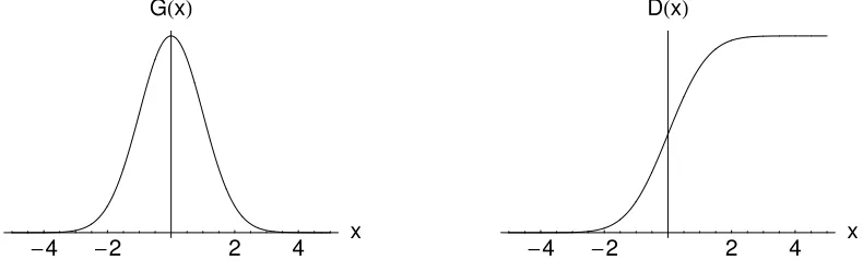
whereG(x), as shown in the plot below, gives the probability that a variate with a Gaussian distribution takes on a value in the range [x, x + dx]. Statisticians commonly call this distribution the normal distribution and, because of its shape, social scientists refer to it as the “bell curve.” G(x) has been normalized so that the accumulated area under the curve between−∞ ≤ x≤ +∞totals to unity. A cumulative distribution function, which totals the area under the normalized distribution curve is available and can be plotted as shown below.

-4 -2 2 4

x G_Hx_L

-4 -2 2 4

x DH_xL

Figure 2.1: Plot of Gaussian Function and Cumulative Distribution Function

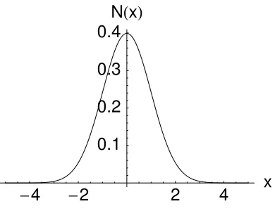
When the mean is set to zero (µ = 0) and the standard deviation or variance is set to unity (σ = 1), we get the familiar normal distribution

G(x) = √1

2π e −x2_/2

dx (1.2)

which is shown in the curve below. The normal distribution function N(x) gives the prob-ability that a variate assumes a value in the interval [0, x]

N(x) = √1

2π

Z x

0

-4 -2 2 4 x 0.1

0.2 0.3 0.4

NHxL

Figure 2.2: Plot of the Normalized Gaussian Function

Gaussian distributions have many convenient properties, so random variates with unknown distributions are often assumed to be Gaussian, especially in physics, astronomy and various aspects of engineering. Many common attributes such as test scores, height, etc., follow roughly Gaussian distributions, with few members at the high and low ends and many in the middle.

Computer Algebra Systems

Function Maple Mathematica

Probability Density Function statevalf[pdf,dist](x) PDF[dist, x]

- frequency of occurrence at x

Cumulative Distribution Function statevalf[cdf,dist](x) CDF[dist, x]

- integral of probability

density function up to x dist =normald[µ, σ] dist =NormalDistribution[µ, σ]

µ= 0 (mean) µ= 0 (mean)

σ = 1 (std. dev.) σ = 1 (std. dev.)

Potential Applications

Error Function

The error function is obtained by integrating the normalized Gaussian distribution.

erf x = √2 π

Z x

0

e−t2 dt (1.4)

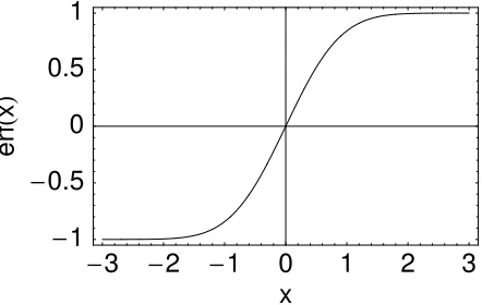
where the coefficient in front of the integral normalizes erf (∞) = 1. A plot of erf x over the range −3 ≤ x≤ 3 is shown as follows.

-3 -2 -1 0 1 2 3

x

-1 -0.5

0 0.5 1

erf

H

x

L

Figure 2.3: Plot of the Error Function

The error function is defined for all values ofx and is considered an odd function inx since

erf x =−erf (−x).

The error function can be conveniently expressed in terms of other functions and series as follows:

erf x = √1 π γ

₁

2, x

2

(1.5)

= √2x π M

1 2,

3 2,−x

2

= √2x π e

−x2 _M

1,3

2, x

2

(1.6)

= √2 π

∞

X

n=0

(−1)n_x2n+1

n!(2n+ 1) (1.7)

Computer Algebra Systems

Function Maple Mathematica

Error Function erf(x) Erf[x]

Complementary Error Function erfc(x) Erfc[x]

Inverse Error Function fslove(erf(x)=s) InverseErf[s]

Inverse Complementary fslove(erfc(x)=s) InverseErfc[s]

Error Function

where sis a numerical value and we solve for x

Potential Applications

1. Diffusion: Transient conduction in a semi-infinite solid is governed by the diffusion equation, given as

∂2_T ∂x2 =

1

α ∂T

∂t

where α is thermal diffusivity. The solution to the diffusion equation is a function of either the erf x or erfc x depending on the boundary condition used. For instance, for constant surface temperature, where T(0, t) = Ts

T(x, t)−Ts

Ti−Ts

= erfc

_x

2√αt

complementary Error Function

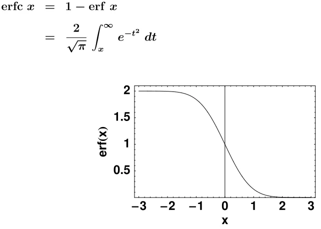
The complementary error function is defined as

erfcx = 1−erf x

= √2 π

Z ∞

x

e−t2 dt (1.8)

-3 -2 -1 0 1 2 3

x 0.5

1 1.5 2

erf

H

x

L

Figure 2.4: Plot of the complementary Error Function

and similar to the error function, the complementary error function can be written in terms of the incomplete gamma functions as follows:

erfcx = √1 π Γ

₁

2, x

2

(1.9)

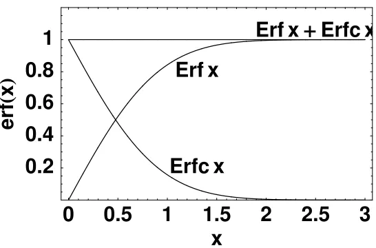
As shown in Figure 2.5, the superposition of the error function and the complementary error function when the argument is greater than zero produces a constant value of unity.

Potential Applications

1. Diffusion: In a similar manner to the transient conduction problem described for the error function, the complementary error function is used in the solution of the diffusion equation when the boundary conditions are constant surface heat flux, whereqs =q0

T(x, t)−Ti =

2q0(αt/π)1/2

k exp

_−x2

4αt

− q0x k erfc

_x

2√αt

0

0.5

1

1.5

2

2.5

3

x

0.2

0.4

0.6

0.8

1

erf

H

x

L

Erf x

+

Erfc x

Erf x

Erfc x

Figure 2.5: Superposition of the Error and complementary Error Functions

and surface convection, where −k ∂T ∂x

x=0

= h[T∞−T(0, t)]

T(x, t)−Ti

T∞−Ti

= erfc

_x

2√αt

−

exp

_hx

k +

h2_αt k2

"

erfc x 2√αt +

h√αt

k

Relations and Selected Values of Error Functions

erf (−x) = −erf x erfc (−x) = 2−erfcx

erf 0 = 0 erfc 0 = 1

erf ∞ = 1 erfc∞ = 0

erf (−∞) = −1

Z ∞

0

erfc x dx = 1/√π

Z ∞

0

erfc2 x dx = (2−√2)/√π

Ten decimal place values for selected values of the argument appear in Table 2.1.

Table 2.1 Ten decimal place values of erf x

x erf x x erf x

0.0 0.00000 00000 2.5 0.99959 30480

0.5 0.52049 98778 3.0 0.99997 79095

1.0 0.84270 07929 3.5 0.99999 92569

1.5 0.96610 51465 4.0 0.99999 99846

Approximations

Power Series for Small x (x < 2)

Since

erf x = √2 π

Z x

0

e−t2 dt = √2 π Z x 0 ∞ X n=0

(−1)nt2n

n! dt (1.10)

and the series is uniformly convergent, it may be integrated term by term. Therefore

erf x = √2 π

∞

X

n=0

(−1)n_x2n+1

(2n+ 1)n! (1.11)

= √2 π

_x

1·0! −

x3

3·1! +

x5

5·2! −

x7

7·3! +

x9

9·4! − · · ·

(1.12)

Asymptotic Expansion for Large x (x >2)

Since

erfcx = √2 π

Z ∞

x

e−t2 dt = √2 π

Z ∞

x

1

t e −t2

t dt

we can integrate by parts by letting

u = 1

t dv = e

−t2

d dt

du = −t−2 _{dt v = −}1

2 e

−t2

therefore

Z ∞

x

1

t e −t2

t dt=

uv ∞ x − Z ∞ x

v du=

− 1

2te −t2

∞ x − Z ∞ x 1 2

e−t2

Thus

erfcx = √2 π

(

1

2xe −x2

− 1

2

Z ∞

x

e−t2

t2 dt

)

(1.13)

Repeating the process n times yields

√ π

2 erfcx = 1

2e

−x21

x −

1

2x3 +

1·3

22_x5 − · · ·+ (−1)

n−11·3· · ·(2n−3)

2n−1_x2n−1

+

+(−1)n1·3· · ·(2n−1) 2n

Z ∞

x

e−t2

t2n dt (1.14)

Finally we can write

√

πxex2erfcx = 1 +

∞

X

n=1

(−1)n1·3·5· · ·(2n−1)

(2x2₎n (1.15)

This series does not converge, since the ratio of thenth_{term to the(n−1)}th_{does not remain} less than unity as nincreases. However, if we take n terms of the series, the remainder,

1·3· · ·(2n−1)

2n

Z ∞

x

e−t2

t2n dt

is less than the nth term because

Z ∞

x

e−t2

t2n dt < e

−x2

<

Z ∞

0 dt

t2n

We can therefore stop at any term taking the sum of the terms up to this term as an approximation of the function. The error will be less in absolute value than the last term retained in the sum. Thus for large x, erfc x may be computed numerically from the asymptotic expansion.

√

πxex2erfcx = 1 +

∞

X

n=1

(−1)n1·3·5· · ·(2n−1) (2x2₎n

= 1− 1

2x2 +

1·3

(2x2₎2 −

1·3·5

Some other representations of the error functions are given below:

erf x = √2 πe

−x2

∞

X

n=0

x2n+1

(3/2)n (1.17)

= √2x

π M

1

2, 3

2,−x

2

(1.18)

= √2x πe

−x2

M

1,3

2, x

2

(1.19)

= √1 π γ

₁

2, x

2

(1.20)

erfcx = √1 π Γ

₁

2, x

2

(1.21)

The symbols γ and Γ represent the incomplete gamma functions, and M denotes the con-fluent hypergeometric function or Kummer’s function.

Derivatives of the Error Function

d

dxerf x=

2

√ πe

−x2

= d dx ₂ √ π Z x 0

e−t2dt

(1.22)

Use of “Leibnitz” rule of differentiation of integrals gives:

d2

dx2erfc x= d

dx

2

√ πe

−x2

=−√2

π(2x)e −x2

(1.23)

d3

dx3erfc x= d

dx

−√2

π(2x)e −x2

= √2 π(4x

2_−2)e−x2

(1.24)

In general we can write

dn+1

dxn+1erf x = (−1)

n _√2

πHn(x)e −x2

(n = 0,1,2. . .) (1.25)

Repeated Integrals of the Complementary Error Function

inerfc x=

Z ∞

x

in−1erfct dt n= 0,1,2, . . . (1.26)

where

i−1erfcx = √2 πe

−x2

(1.27)

i0erfcx = erfc x (1.28)

i1erfcx = ierfcx =

Z ∞

x

erfc t dt

= √1

π exp(−x 2

)−x erfc x (1.29)

i2erfcx =

Z ∞

x

i erfct dt

= 1 4

(1 + 2x2) erfc x− √2

π xexp(−x 2₎

= 1

4 [erfc x−2x · ierfc x] (1.30)

The general recurrence formula is

2nin erfcx =in−2 erfcx−2xin−1 erfcx (n= 1,2,3, . . .) (1.31)

Therefore the value at x= 0 is

inerfc 0− 1

2n _Γ

1 + n 2

(n= −1,0,1,2,3, . . .) (1.32)

It can be shown thaty = in _{erfcx is the solution of the differential equation}

d2_y dx2 + 2x

dy

The general solution of

y00+ 2xy0−2ny = 0 − ∞ ≤ x≤ ∞ (1.34)

is of the form

y =Ainerfc x+Binerfc (−x) (1.35)

Derivatives of Repeated Integrals of the Complementary Error

Function

d

dx[i

n_{erfc x] = (−1)}n−1

erfcx (n = 0,1,2,3. . .) (1.36)

dn

dxn

h

Some Integrals Associated with the Error Function

Z x2

0

e−t √

t dt = √

π erf x (1.38)

Z x

0

e−t y dt =

√ π

2y erf x (1.39)

Z 1

0

e−t2 x2

1 +t2 dt = π

2 e

x2

1− {erf x}2

(1.40)

Z ∞

0

e−t x

√

y+t dt = √

π √

xe

xy_{erfc (}√_{xy) x >0 (1.41)}

Z ∞

0

e−t2_x

t2 _+y2 dt = π

2ye

xy2

erfc (√xy) x >0, y > 0 (1.42)

Z ∞

0

e−tx

(t+y)√t dt = π √

ye

xy _{erfc (xy) x >0, y 6= 0 (1.43)}

Z ∞

0

e−t xerf (pyt) dt =

√ y

x (x+y)

−1/2 _{(x+y) > 0 (1.44)}

Z ∞

0

e−t xerf (py/t dt = 1

xe

−2√xy _{x > 0, y > 0 (1.45)}

Z ∞

−a

erfc (t) dt = ierfc (a) + 2a = ierfc (−a) (1.46)

Z a

−a

erf (t) dt = 0 (1.47)

Z a

−a

erfc(t) dt = 2a (1.48)

Z ∞

−a

ierfc (t) dt = i2 erfc (−a) = 1

2 +a−i

2 _{erfc (a) (1.49)}

Z ∞

a

in erfc

t+c b

dt = bin+1 erfc

a+c b

Numerical Computation of Error Functions

The power series form of the error function is not recommended for numerical computations when the argument approaches and exceeds the value x = 2 because the large alternat-ing terms may cause cancellation, and because the general term is awkward to compute recursively. The function can, however, be expressed as a confluent hypergeometric series.

erf x = √2 πx e

−x2

M

1,3

2, x

2

(1.51)

in which all terms are positive, and no cancellation can occur. If we write

erf x =b ∞

X

n=0

an 0≤ x ≤ 2 (1.52)

with

b = √2x π e

−x2

a0 = 1 an =

x2

(2n+ 1)/2 an−1 n ≥1

then erf x can be computed very accurately (e.g. with an absolute error less that 10−9). Numerical experiments show that this series can be used to compute erf x up to x = 5

to the required accuracy; however, the time required for the computation of erf x is much greater due to the large number of terms which have to be summed. Forx ≥ 2an alternate method that is considerably faster is recommended which is based upon the asymptotic expansion of the complementary error function.

erfcx = √2 π

Z ∞

x

e−t2 dt

= e

−x2

√

πx2 Fo

₁

2,1,− 1

x2

x→ ∞ (1.53)

√

πex2erfcx = 1

x+ 1/2

x+ 1

x+ 3/2

x+ 2

x+ 5/2

x+. . .

x >0 (1.54)

which for convenience will be written as

erfcx = e

−x2

√ π

1

x+ 1/2

x+ 1

x+ 3/2

x+ 2

x+ · · ·

x >0 (1.55)

It can be demonstrated experimentally that for x ≥ 2 the 16th approximant gives erfc x

with an absolute error less that 10−9. Thus we can write

erfcx = e

−x2

√ π

₁

x+ 1/2

x+ 1

x+ 3/2

x+ · · · 8

x

x ≥2 (1.56)

Rational Approximations of the Error Functions (0

≤

x <

∞)

Numerous rational approximations of the error functions have been developed for digital computers. The approximations are often based upon the use of economized Chebyshev polynomials and they give values of erf x from 4 decimal place accuracy up to 24 decimal place accuracy.

Two approximations by Hastings et al.11 _{are given below.}

erf x = 1−[t(a1+t(a2 +a3t))]e−x

2

+(x) 0 ≤ x (1.57)

where

t = 1

1 +px

and the coefficients are

p = 0.47047

a1 = 0.3480242

a2 = −0.0958798

a3 = 0.7478556

This approximation has a maximum absolute error of |(x)| <2.5×10−5.

Another more accurate rational approximation has been developed for example

erf x = 1−[t(a1+t(a2 +t(a3+t(a4 +a5t))))]e−x

2

+(x) (1.58)

where

t = 1

and the coefficients are

p = 0.3275911

a1 = 0.254829592

a2 = −0.284496736

a3 = 1.421413741

a4 = −1.453152027

a5 = 1.061405429

Assigned Problems

Problem Set for Error and Due Date: February 12, 2004 Complementary Error Function

1. Evaluate the following integrals to four decimal places using either power series, asymp-totic series or polynomial approximations:

a)

Z 2

0

e−x2 dx b)

Z 0.002

0.001

e−x2 dx

c) √2 π

Z ∞

1.5

e−x2 dx d) √2

π

Z 10

5

e−x2 dx

e)

Z 1.5

1

1

2e

−x2

dx f) r 2 π Z ∞ 1 1 2e

−x2

dx

2. The value of erf 2 is 0.995 to three decimal places. Compare the number of terms required in calculating this value using:

a) the convergent power series, and b) the divergent asymptotic series.

Compare the approximate errors in each case after two terms; after ten terms.

3. For the functionierfc(x)compute to four decimal places whenx = 0, 0.2, 0.4, 0.8,

and 1.6.

4. Prove that

i) √π erf (x) = γ

₁

2, x

2

ii) √π erfc(x) = Γ

₁

2, x

2

where γ

₁

2, x

2

and Γ

₁

2, x

2

γ(a, y) =

Z y

0

e−uua−1 du

and

Γ(a, y) =

Z ∞

y

e−uua−1 du

5. Show that θ(x, t) = θ0 erfc(x/2√αt) is the solution of the following diffusion problem:

∂2_θ ∂x2 =

1

α ∂θ

∂t x≥ 0, t > 0

and

θ(0, t) = θ0, constant

θ(x, t) → 0 as x→ ∞

6. Given θ(x, t) = θ0 erf x/2√αt:

i) Obtain expressions for ∂θ

∂t and ∂θ

∂x at anyx and allt > 0

ii) For the function

√ π

2

x

θ0 ∂θ

∂x

show that it has a maximum value when x/2√αt = 1/√2 and the maximum value is 1/√2e.

7. Given the transient point source solution valid within an isotropic half space

T = q

2πkr erfc(r/2 √

derive the expression for the transient temperature rise at the centroid of a circular area (πa2_{) which is subjected to a uniform and constant heat fluxq. Superposition of}

point source solutions allows one to write

T0 =

Z a

0

Z 2π

0

T dA

8. For a dimensionless time F o < 0.2 the temperature distribution within an infinite plate −L≤ x≤ L is given approximately by

T(ζ, F o)−Ts

T0−Ts

= 1−

erfc 1−ζ

2√F o + erfc

1 +ζ

2√F o

for 0 ≤ζ ≤ 1 where ζ =x/L and F o= αt/L2_.

Obtain the expression for the mean temperature (T(F o)−Ts)/(T0 −Ts) where

T =

Z 1

0

T(ζ, F o) dζ

The initial and surface plate temperature are denoted by T0 and Ts, respectively.

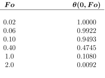
9. Compare the approximate short time (F o < 0.2) solution:

θ(ζ, F o) = 1− 3

X

n=1

(−1)n+1

erfc(2n−1)−ζ

2√F o + erfc

(2n−1) +ζ

2√F o

and the approximate long time (F o > 0.2) solution

θ(ζ, F o) =

3

X

n=1

2(−1)n+1 δn

e−δ2nF o _cos(δ

nζ)

with δn = (2n−1)π/2.

Table 1: Exact values ofθ(0, F o) for the Infinite Plate

F o θ(0, F o)

0.02 1.0000

0.06 0.9922

0.10 0.9493

0.40 0.4745

1.0 0.1080

References

1. Abramowitz, M. and Stegun, I.A., Handbook of Mathematical Functions, Dover, New York, 1965.

2. Fletcher, A., Miller, J.C.P., Rosehead, L. and Comrie, L.J., An Index of Mathematical Tables, Vols. 1 and 2, 2 edition, Addison-Wesley, Reading, Mass., 1962.

3. Hochsadt, H., Special Functions of Mathematical Physics, Holt, Rinehart and Win-ston, New York, 1961.

4. Jahnke, E., Emdw, F. and Losch, F., Tables of Higher Functions, 6th Edition, McGraw-Hill, New York, 1960.

5. Lebedev, A.V. and Fedorova, R.M., A Guide to Mathematical Tables, Pergamon Press, Oxford, 1960.

6. Lebedev, N.N.,Special Functions and Their Applications, Prentice-Hall, Englewood Cliffs, NJ, 1965.

7. Magnus, W., Oberhettinger, F. and Soni, R.P.,Formulas and Theorems for the Functions of Mathematical Physics, 3rd Edition, Springer-Verlag, New York, 1966.

8. Rainville, E.D., Special Functions, MacMillan, New York, 1960.

9. Sneddon, I.N., Special Functions of Mathematical Physics and Chemistry, 2nd Edi-tion, Oliver and Boyd, Edinburgh, 1961.

10. National Bureau of Standards, Applied Mathematics Series 41, Tables of Error Function and Its Derivatives, 2nd Edition, Washington, DC, US Government Printing Office, 1954.

Chebyshev Polynomials

Reading Problems

Differential Equation and Its Solution

The Chebyshev differential equation is written as

(1−x2) d

2_y dx2 −x

dy

dx +n

2 _{y = 0 n = 0,1,2,3, . . .}

If we let x= cost we obtain

d2_y dt2 +n

2_{y = 0}

whose general solution is

y =Acosnt+Bsinnt

or as

y =Acos(ncos−1x) +Bsin(ncos−1x) |x|< 1

or equivalently

y =ATn(x) +BUn(x) |x| <1

If we let x= cosht we obtain

d2y dt2 −n

2_{y = 0}

whose general solution is

y =Acoshnt+Bsinhnt

or as

y =Acosh(ncosh−1x) +Bsinh(ncosh−1x) |x| > 1

or equivalently

y =ATn(x) +BUn(x) |x| >1

The function Tn(x) is a polynomial. For |x|< 1 we have

Tn(x) +iUn(x) = (cost+isint)n =

x+ip1−x2n

Tn(x)−iUn(x) = (cost−isint)n =

x−ip1−x2n

from which we obtain

Tn(x) =

1

2

h

x+ip1−x2n_+x−ip_1−x2ni

For|x|> 1 we have

Tn(x) + Un(x) = ent =

x±px2 ₋₁n

Tn(x)−Un(x) = e−nt =

x∓px2 ₋₁n

Chebyshev Polynomials of the First Kind of Degree

n

The Chebyshev polynomials Tn(x)can be obtained by means of Rodrigue’s formula

Tn(x) =

(−2)n_n!

(2n)!

p

1−x2 d

n

dxn (1−x

2₎n−1/2 _{n = 0,1,2,3, . . .}

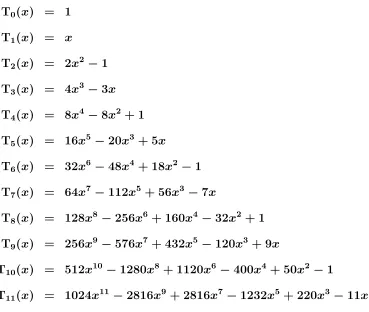
Table 1: Chebyshev Polynomials of the First Kind

T0(x) = 1

T1(x) = x

T2(x) = 2x2 −1

T3(x) = 4x3 −3x

T4(x) = 8x4 −8x2 + 1

T5(x) = 16x5 −20x3+ 5x

T6(x) = 32x6 −48x4+ 18x2−1

T7(x) = 64x7 −112x5+ 56x3−7x

T8(x) = 128x8 −256x6+ 160x4 −32x2 + 1

T9(x) = 256x9 −576x7+ 432x5 −120x3 + 9x

T10(x) = 512x10−1280x8 + 1120x6 −400x4+ 50x2−1

Table 2: Powers of x as functions of Tn(x)

1 = T0

x = T1

x2 = 1

2(T0+T2)

x3 = 1

4(3T1+T3)

x4 = 1

8(3T0+ 4T2 +T4)

x5 = 1

16(10T1 + 5T3 +T5)

x6 = 1

32(10T0 + 15T2 + 6T4+T6)

x7 = 1

64(35T1 + 21T3 + 7T5+T7)

x8 = 1

128(35T0 + 56T2 + 28T4 + 8T6 +T8)

x9 = 1

256(126T1 + 84T3+ 36T5 + 9T7+T9)

x10 = 1

512(126T0 + 210T2+ 120T4 + 45T6+ 10T8 +T10)

x11 = 1

Generating Function for

T

(

x

)

The Chebyshev polynomials of the first kind can be developed by means of the generating function

1−tx

1−2tx+t2 = ∞

X

n=0

Tn(x)tn

Recurrence Formulas for

T

(

x

)

When the first two Chebyshev polynomials T0(x) and T1(x) are known, all other

polyno-mials Tn(x), n≥ 2 can be obtained by means of the recurrence formula

Tn+1(x) = 2xTn(x)−Tn−1(x)

The derivative of Tn(x)with respect to xcan be obtained from

(1−x2)T_n0(x) = −nxTn(x) +nTn−1(x)

Special Values of

T

(

x

)

The following special values and properties of Tn(x) are often useful:

Tn(−x) = (−1)nTn(x) T2n(0) = (−1)n

Tn(1) = 1 T2n+1(0) = 0

Orthogonality Property of

T

(

x

)

We can determine the orthogonality properties for the Chebyshev polynomials of the first kind from our knowledge of the orthogonality of the cosine functions, namely,

Z π

0

cos(mθ) cos(n θ) dθ =

     

    

0 (m 6=n)

π/2 (m =n 6= 0)

π (m =n = 0)

Then substituting

Tn(x) = cos(nθ)

cosθ = x

to obtain the orthogonality properties of the Chebyshev polynomials:

Z 1

−1

Tm(x) Tn(x) dx

√

1−x2 =

     

    

0 (m6=n)

π/2 (m=n 6= 0)

π (m=n = 0)

We observe that the Chebyshev polynomials form an orthogonal set on the interval −1 ≤ x ≤1 with the weighting function (1−x2₎−1/2

Orthogonal Series of Chebyshev Polynomials

An arbitrary function f(x) which is continuous and single-valued, defined over the interval

−1 ≤ x≤ 1, can be expanded as a series of Chebyshev polynomials:

f(x) = A0T0(x) +A1T1(x) +A2T2(x) +. . .

=

∞

X

n=0

where the coefficients An are given by

A0 =

1

π

Z 1

−1

f(x) dx √

1−x2 n = 0

and

An =

2

π

Z 1

−1

f(x) Tn(x)dx

√

1−x2 n= 1,2,3, . . .

The following definite integrals are often useful in the series expansion of f(x):

Z 1

−1 dx √

1−x2 = π

Z 1

−1

x3 _dx √

1−x2 = 0

Z 1

−1

x dx √

1−x2 = 0

Z 1

−1

x4 dx √

1−x2 =

3π

8

Z 1

−1

x2 _dx √

1−x2 = π

2

Z 1

−1

x5 _dx √

1−x2 = 0

Chebyshev Polynomials Over a Discrete Set of Points

A continuous function over a continuous interval is often replaced by a set of discrete values of the function at discrete points. It can be shown that the Chebyshev polynomials Tn(x) are orthogonal over the following discrete set of N + 1 points xi, equally spaced on θ,

θi = 0,

π

N,

2π

N, . . .(N −1) π

N, π

where

xi = arccos θi

1

2Tm(−1)Tn(−1)+

N−1

X

i=2

Tm(xi)Tn(xi)+

1

2Tm(1)Tn(1) =

     

    

0 (m6= n)

N/2 (m= n6= 0)

N (m= n= 0)

The Tm(x) are also orthogonal over the following N points ti equally spaced,

θi =

π

2N,

3π

2N,

5π

2N, . . . ,

(2N −1)π

2N

and

ti = arccos θi

N

X

i=1

Tm(ti)Tn(ti) =

     

    

0 (m6=n)

N/2 (m=n 6= 0)

N (m=n = 0)

The set of points ti are clearly the midpoints in θ of the first case. The unequal spacing of the points inxi(N ti) compensates for the weight factor

W(x) = (1−x2)−1/2

Additional Identities of Chebyshev Polynomials

The Chebyshev polynomials are both orthogonal polynomials and the trigonometriccosnx

functions in disguise, therefore they satisfy a large number of useful relationships.

The differentiation and integration properties are very important in analytical and numerical work. We begin with

Tn+1(x) = cos[(n+ 1) cos−1x]

and

Tn−1(x) = cos[(n−1) cos−1x]

Differentiating both expressions gives

1

(n+ 1)

d[Tn+1(x)]

dx =

−sin[(n+ 1) cos−1x −√1−x2

and

1

(n−1)

d[Tn−1(x)]

dx =

−sin[(n−1) cos−1x −√1−x2

Subtracting the last two expressions yields

1

(n+ 1)

d[Tn+1(x)]

dx −

1

(n−1)

d[Tn−1(x)]

dx =

sin(n+ 1)θ−sin(n−1)θ

sinθ

or

T_n0₊₁(x) (n+ 1) −

T_n0₋₁(x)

(n−1) =

2 cosnθ sinθ

Therefore

T₂0(x) = 4T1

T₁0(x) = T0

T₀0(x) = 0

We have the formulas for the differentiation of Chebyshev polynomials, therefore these for-mulas can be used to develop integration for the Chebyshev polynomials:

Z

Tn(x)dx =

1

2

_T

n+1(x)

(n+ 1) −

Tn−1(x)

(n−1)

+C n≥ 2

Z

T1(x)dx =

1

4T2(x) +C

Z

T0(x)dx = T1(x) +C

The Shifted Chebyshev Polynomials

For analytical and numerical work it is often convenient to use the half interval 0 ≤ x≤ 1

instead of the full interval−1 ≤ x≤ 1. For this purpose the shifted Chebyshev polynomials are defined:

T_n∗(x) = Tn ∗(2x−1)

Thus we have for the first few polynomials

T₀∗ = 1

T₁∗ = 2x−1

T₂∗ = 8x2−8x+ 1

T₃∗ = 32x3−48x2 + 18x−1

and the following powers of xas functions of T_n∗(x);

1 = T₀∗

x = 1

2(T

∗ 0 +T

∗ 1)

x2 = 1 8(3T

∗ 0 + 4T

∗ 1 +T

∗ 2)

x3 = 1 32(10T

∗

0 + 15T ∗ 1 + 6T

∗ 2 +T

∗ 3)

x4 = 1

128(35T

∗

0 + 56T ∗

1 + 28T ∗ 2 + 8T

∗ 3 +T

∗ 4)

The recurrence relationship for the shifted polynomials is:

T_n∗₊₁(x) = (4x−2)T_n∗(x)−T_n∗₋₁(x) T₀∗(x) = 1

or

xT_n∗(x) = 1 4T

∗

n+1(x) +

1

2T

∗

n(x) +

1

4T

∗

n−1(x)

where

T_n∗(x) = cosncos−1(2x−1) =Tn(2x−1)

Expansion of

x

in a Series of

T

(

x

)

A method of expanding xn in a series of Chebyshev polynomials employes the recurrence relation written as

xTn(x) =

1

2[Tn+1(x) +Tn−1(x)] n= 1,2,3. . .

To illustrate the method, considerx4

x4 = x2(xT1) = x2

2 [T2 +T0] =

x

4[T1 +T3+ 2T1]

= 1

4[3xT1 +xT3] = 1

8[3T0+ 3T2 +T4+T2]

= 1 8T4 +

1

2T2 + 3

8T0

This result is consistent with the expansion of x4 _{given in Table 2.}

Approximation of Functions by Chebyshev Polynomials

Sometimes when a function f(x) is to be approximated by a polynomial of the form

f(x) =

∞

X

n=0

anxn+EN(x) |x| ≤ 1

where |En(x)| does not exceed an allowed limit, it is possible to reduce the degree of the polynomial by a process called economization of power series. The procedure is to convert the polynomial to a linear combination of Chebyshev polynomials:

N

X

n=0

anxn = N

X

n=0

bnTn(x) n= 0,1,2, . . .

It may be possible to drop some of the last terms without permitting the error to exceed the prescribed limit. Since |Tn(x)| ≤ 1, the number of terms which can be omitted is determined by the magnitude of the coefficient b.

The Chebyshev polynomials are useful in numerical work for the interval −1 ≤ x ≤ 1

because

1. |Tn(x)] ≤ 1 within−1 ≤ x≤ 1

3. The maxima and minima are spread reasonably uniformly over the interval

−1 ≤ x≤ 1

4. All Chebyshev polynomials satisfy a three term recurrence relation.

5. They are easy to compute and to convert to and from a power series form.

These properties together produce an approximating polynomial which minimizes error in its application. This is different from the least squares approximation where the sum of the squares of the errors is minimized; the maximum error itself can be quite large. In the Chebyshev approximation, the average error can be large but the maximum error is minimized. Chebyshev approximations of a function are sometimes said to be mini-max approximations of the function.

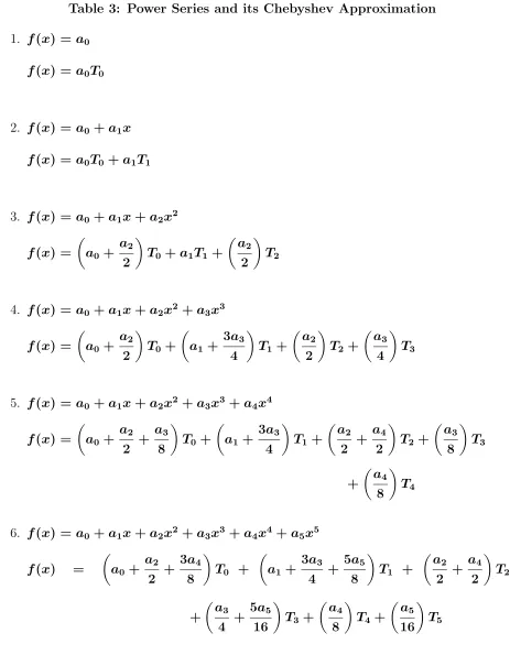
Table 3: Power Series and its Chebyshev Approximation

1. f(x) = a0

f(x) = a0T0

2. f(x) = a0 +a1x

f(x) = a0T0+a1T1

3. f(x) = a0 +a1x+a2x2

f(x) =

a0 + a2

2

T0 +a1T1 +

_a

2

2

T2

4. f(x) = a0 +a1x+a2x2 +a3x3

f(x) =

a0 + a2

2

T0 +

a1+

3a3

4

T1+

_a

2

2

T2 +

_a

3

4

T3

5. f(x) = a0 +a1x+a2x2 +a3x3 +a4x4

f(x) =

a0 + a2

2 +

a3

8

T0 +

a1+

3a3

4

T1+

_a 2 2 + a4 2

T2+

_a 3 8 T3 + _a 4 8 T4

6. f(x) = a0 +a1x+a2x2 +a3x3 +a4x4+a5x5

f(x) =

a0+ a2

2 + 3a4

8

T0 +

a1 +

3a3

4 + 5a5

8

T1 +

_a 2 2 + a4 2 T2 + _a 3 4 + 5a5

16

T3 +

_a

4

8

T4 +

_a

5

16

Table 4: Formulas for Economization of Power Series

x = T1

x2 = 1

2(1 +T2)

x3 = 1

4(3x+T3)

x4 = 1 8(8x

2 _{−1 +T} 4)

x5 = 1 16(20x

3 _−5x+T 5)

x6 = 1 32(48x

4 _−18x2_{+ 1 +T} 6)

x7 = 1

64(112x

5 _−56x3_{+ 7x+T} 7)

x8 = 1

128(256x

6 _−160x4_{+ 32x}2_{−1 +T} 8)

x9 = 1

256(576x

7 _−432x5_{+ 120x}3_−9x+T 9)

x10 = 1

512(1280x

8_−1120x6 _{+ 400x}4 _−50x2 _{+ 1 +T} 10)

x11 = 1

1024(2816x

9_−2816x7 _{+ 1232x}5 _−220x3_{+ 11x+T} 11)

Assigned Problems

Problem Set for Chebyshev Polynomials

1. Obtain the first three Chebyshev polynomials T0(x), T1(x) and T2(x) by means of

the Rodrigue’s formula.

2. Show that the Chebyshev polynomial T3(x) is a solution of Chebyshev’s equation of

order 3.

3. By means of the recurrence formula obtain Chebyshev polynomials T2(x) and T3(x)

given T0(x) and T1(x).

4. Show that Tn(1) = 1and Tn(−1) = (−1)n

5. Show that Tn(0) = 0if nis odd and (−1)n/2 if n is even.

6. Setting x = cosθ show that

Tn(x) =

1

2

h

x+ip1−x2n _+x−ip_1−x2ni

where i =√−1.

7. Find the general solution of Chebyshev’s equation for n = 0.

8. Obtain a series expansion for f(x) = x2 _{in terms of Chebyshev polynomialsT}

n(x),

x2 =

3

X

n=0

AnTn(x)