GSJ: Volume 7, Issue 7, July 2019, Online: ISSN 2320-9186
www.globalscientificjournal.com
S
IMPLE AND
E
FFICIENT
D
ESIGN OF A
M
ODEL
-
FREE
CONTROLLER BASED ON LAG
/
LEAD COMPENSATOR
David Monjengue
ABSTRACT
This paper presents a new approach for designing Model-free Controller, based on lag/lead compensator. The design objectives were to have a model-free controller, which is simple easy to tune. The proposed controller has showed efficiency in term of performances and design time requirements. Although, the model-free controllers presented in the literature are only focus in tracking objectives, this Model-free controller is also able to control the system performances such as settling time, rising time, error and overshoot, by tuning the two parameters that it is composed of. The absence of model make it able to be applied in different systems and fields.
Introduction
In order to understand and better control a plant, one have to know the exact characteristics of the plant. For that, a mathematical representation of the plant is required, with a precise mathematical model, there is a large range of efficient controllers available in the literature. In practice, an exact model of a plant is very difficult to have, due to the presence of unavoidable nonlinearities affecting the plant, such as friction, ageing of the system, heat effects, etc. [1].
The need to design controllers that are robust to system uncertainties is crucial because, the various parameters that compose a system are affected by many external factors such as presence of magnetic field, temperature, pressure, load variation, wind, dust etc. All these factors affect the system
parameters in such a way that, it is very difficult to know exactly the parameters values, but only an interval in which each parameter is located. G. Qi stated: “In practice, the model of a plant is usually unknown or only partially unknown” *2+.
Some researchers tented to linearize the nonlinearities around an operation point, again this solution is only accurate around the operative point. For system with large operative range this solution does not work. Nonlinear control strategies such as backstepping [3] and sliding mode [4] were developed, in order to have a precise control of nonlinear systems. Nevertheless, they are rarely employed in industry because of their requirement of a precise mathematical modeling to achieve an accurate control and their complexity of implementation and control gain tuning [5].
The most popular controller used in industry is still PID controller, because of its simple structure and easy parameters tuning. P. Gédouin stated that “to realize a process control, the part of process modeling represents 90% of project global time and requires a true know-how in control and about the process to be controlled” *6+.
In this study, we designed a model-free control, which aims is to combine the simplicity and easy tune characteristics of PID control, and the absence of model knowledge of model-free control, in order to reduce the design time, improve the efficiency of the control, and make it easy to tune. The presented model-free control is of a big importance, since many equipment that were only available for specialized areas are being make available to everyone for domestic usage, such as drones, machine tools, robots, DC motors, ROV, etc. These equipment, as there are widely being used by common people, should be highly reliable and easy to tune if necessary to refine the performances.
Model-free control
Model-free (MFC) attempts to internally model the unknown portions of the system, and subsequently eliminate them using the controller output [1].
replaced by the following equation, which is only valid during a very short period of time [1]:
(1)
is a parameter selected by the practitioner, it should be low usually v (first or second order differential equation).
F: the unknown plant constant parameter and the effect of perturbation on the plant. : the control law.
a non-physical constant parameters selected by the practitioner such that are of the same magnitude.
F: estimated via the measure of and (actually the past values of and .
To derive the control law, the system is closed via . The control law is given :
̇ ∫ ̇
(2)
The estimate of F is given by M.Fliess [8] by:
∫ [ ] (3)
One particular caveat of MFC is that it demonstrates poor performance for unknown plants that are Non-minimal phase [7]. Besides that, the MFC with ultra-local model needs to estimate the internal model. The estimation takes time, thus it will induce a supplementary delay to the system
performances.
In this study, we designed a model-free control, which avoid the internal plant estimation, and is of simple structure. By simple structure, we understand easily realizable physiscally, as PID, Lag/lead controllers.
Model-free lag/lead compensator (MFCLL)
In the MFCLL, we observe the system closed loop behavior and we incorporate a lag/lead compensator which role is to feed the closed loop system with the appropriate signal in order to produce the desired performances, as illustrated in the below figure.
Y(S)
U(S) Gain
Plant
GNL(S)
K 𝒔 𝒂 𝒃
𝒔 𝒂
Figure 1: MFCLL Principle
Assumption: The closed-loop system is stable.
The transfer function of fig.1 is:
(4) Stability Analysis The system is stable:
If { (5)
is stable (our initial assumption)
is stable if
The compensator can be a Lead or a Lag compensator depending on the value of the parameters a and b. Determining Lead-lag parameters (a, b)
Applying the final value theorem to (4), and to the Closed-loop alone, we obtain:
(6) (7)
(7) in (6) gives:
(8)
If we want the output ( to follow the reference input ( ), then (8) becomes:
(9)
. The only external parameter to our controller is . When the system operates without any controller then its final value is the value of , assuming the system is stable.
The parameter is then the only parameter necessary to be tuned in order to have the system reach desired final value specifications. The parameter “K”, is intrinsically related to “L”.
The designed controller has the following proprieties:
- a simple structure (easy to implement and only two parameters needs to be tuned);
- does not required to know system parameters, only the final value of the system closed loop; - does not need internal plant estimate.
Simulations
The simulations were conducted using the DC motor control trainer (DCMCT) by Quanser [9], and compare to four different controller which are: PI, LQR (Linear Quadratic Regulator), FCSC (Fixed-weighted Collaborative speed controller, ACSC (adaptive Collaborative Speed Controller). The parameters used for this DC motor are as follow:
Armature inductance (L ) = 0.047 H Armature resistance (R ) = 3.3 Ω Mechanical inertia (J) = 9.64e-6 Kg.m2 Friction coefficient (B) = 1.18e-5 N-m/rad/sec Back emf constant = 0.028 V/rad/sec Motor torque constant = 0.028 N.m/A
The simulation software used was Scilab The open loop transfer function is given by:
(10)
Test 01
MFCLL parameters:
Figure 2: MFCLL simulation with original parameters
From the above figure, we can see that the overshoot is above 50 %, and the settling time is 0.8 seconds, which is very high compare to the others controllers (see table 1, below). The controller parameters need to be tuned in order to improve the system performances.
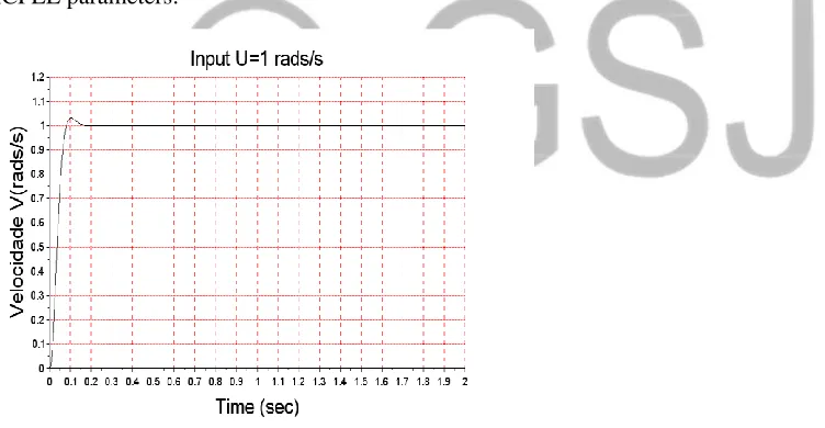
We increase the value of to be 100, in order to increase the settling time and we reduce the value of “K” to be 0.01, in order to reduce the overshoot. The below figure shows the results after the tuning of the MCFLL parameters:
Figure 3: Step response result after tuning of MFCLL parameters
The below table is a comparative table for the performances of four controllers, PI, LQR, FCSC, ACSC controllers as designed in [9] and the model free controller proposed in this study.
Parameter PI LQR FCSC ACSC MFLL (simulation 1)
a=1, b=0.029, L=0.971, K=0.01
MFLL (simulation 2)
a=100, b=293.92,
L=0.254, K=0.01
Tr (s) 0.43 0.12 0.29 0.14 0.0047 0.051
Ts(s) 0.60 0.23 0.40 0.16 0.3573 0.12
OS(%) 0.57 13.70 5.61 3.06 56 3
Ess (steady State error)
0.39rad/s 3.52rad/s 2.17rad/s 0.91rad/s 0rad/s 0rad/s
second simulation a proportional gain “K” was decreased in order to reduce the overshoot, and the parameter was increased, the result of these modifications shows a very good improvement. The model-free controller has now better performances than the others controllers for the DC motor used.
Conclusion
References
*1+ M. Fliess & C. Join, “Model-free control and Intelligent PID controllers: Towards a possible
trivialization of nonlinear Control?”, Proceedings of the 15th IFAC Symposium on System Identification Saint-Malo, France, July 6-8-2009.
*2+ G. Qi, Z.Chen and Z. Yuan, “Model-free control of affine chaotic systems”, Elsevier, Physiscs Letters A 344 (2005) 189-202.
*3+ M. Smaoui, X. Brun, and D. Thomasset, “A study on tracking position control of electropneumatic system using backstepping design”, Control Engenering Practice, 14(8):923-933, Aug 2006.
[4] A. Levant, “Universal SISO sliding-mode controllers with finite-time convergence”. In IEEE Transaction on Automatic Control Barcelona, Vol. 46, p1447-1451, 2001.
*5+ Y. Xu, E. Bideaux, and D. Thomasset, “Robutness study on the Model-free Control and the control with restricted Model of a high performance Electro-Hydraulic System”. The 13th Scandinavian International Conference on Fluid Power, SICFP2013, June 3-5, 2013, Linköping, Sweden.
*6+ PA. Gédouin, E. Delaleau, JM. Bourgeot, C. join, S. A. Chirani, S. Calloch, “Experimental comparison of classical PID and model-free control: position of a shape memory alloy active spring”. HAL Id: inria-00563941, February 2011.
*7+ A. Y. Zenkov. “The method of dominant polynomials for model-free control of dynamical systems”, Master of science thesis, Northeastern University, Boston, Massachusetts, May 2015.
[8] M. Fliess and C. Join. Model-free control, arXiv: 1305v2 [math.OC] 20 November 2013.
[9] O. SALEEM, K. MAHMOOD-UL-HASAN. “Adaptive collaborative speed control of PMDC motor using hyperbolic secant functions and particle swarm optimization”. Turkish Journal of Electrical Engineering & Computer Sciences (2018) 26: 1612 – 1622 doi:10.3906/elk-1709-54