Comparative study of LTE simulations with the ns-3 and the Vienna simulators

(1)

Comparative study of LTE simulations with the ns-3 and

the Vienna simulators

Thiago Abreu

Université Pierre et Marie

Curie - LIP6 75005, Paris, France

Bruno Baynat

Marouen Gachaoui

LIA/CERI University of Avignon 84000, Avignon, France

Tania Jiménez

LIA/CERI University of Avignon 84000, Avignon, France

Narcisse Nya

ABSTRACT

In this paper we compare two simulators: ns-3 and Vienna, in the context of LTE networks, on four basic scenarios for which well-known analytical results exist. These scenarios differentiate themselves by the nature of the traffic (data or voice) and by the number of sources (infinite or finite). Our goal is twofold. First, by confronting the results of the two simulators with exact results, we can assess the accuracy of both simulators and compare their efficiency. Second, and maybe more importantly, we want to compare the ease of handling and use of both simulators, and list the difficulties encountered in the context of the four basic scenarios, that will necessarily arise in more realistic simulated scenarios, and explain how we worked around the problems. We hope this comparison will help researchers who work on LTE net-works to choose the simulator that best suits their needs.

Keywords

Simulators, ns-3, Vienna, LTE.

1. INTRODUCTION

The Long Term Evolution (LTE) standard, specified by the 3rd Generation Partnership Project (3GPP) in release 8, is the next step forward in cellular 3G services. LTE offers significant improvements over previous technologies such as Global System for Mobile communications (GSM), Univer-sal Mobile Telecommunications System (UMTS) and High-Speed Packet Access (HSPA) by reforming the core network and introducing a novel physical layer. The main reasons of these changes in the Radio Access Network (RAN)

sys-tem design are the need to provide higher spectral efficiency, lower delay and more multi-user flexibility than the currently deployed networks [1].

The Idefix project [2] proposes intelligent network and ser-vice control mechanisms that ensure constancy of QoS in time and space, while maintaining energy consumption at reasonable levels. For this goal there is a strong need for testing the proposed mechanisms and algorithms by sim-ulation. Many options of simulators were studied, among them: ns-3, Vienna, SimuLTE and home-made simulators. The project finally chose to compare ns-3 and Vienna, be-cause they are felt as the best-suited simulators in the con-text of LTE networks. Indeed Vienna is purely dedicated to LTE networks, whereas ns-3 is much more general and is based on standard modules designed to simulate different technologies and scenarios. For our comparison we used the LTE module developed by the LENA Project. This module was designed following the 3GPP LTE standard specifica-tions and is included in the main distribution of the ns-3 latest versions.

In order to provide an efficient and methodic comparison of ns-3 and Vienna LTE simulators, we have chosen to con-sider four basic scenarios, for which exact analytical results exist. These scenarios differentiate themselves by the nature of the traffic (Data or Voice) and by the number of sources (Infinite or Finite). The “Voice Infinite source (VI)” and “Voice Finite source (VF)” scenarios correspond to the well-known Erlang and Engset results, whereas the “Data Infinite source (DI)” and “Data Finite source (DF)” scenarios corre-spond to open and closed Processor Sharing queues. We compared the performance indexes obtained by both simu-lators to the analytical expressions provided by models. The objective was first to assess the accuracy of both simulators, and compare their efficiency in terms of run-time, memory usage and CPU occupation. Our goal was also to confront the ease of handling and use of the two tested simulators and evaluate the efforts that are necessary in both cases to handle more realistic scenarios. Finally we list all the

(2)

ficulties we have encountered in the implementation of our four basic scenarios, and propose possible solutions to work around the problems. We believe that these problems will arise in more complex scenarios and we hope that our so-lutions may be helpful for researchers that will have to use simulation in the context of LTE networks.

To the best of our knowledge this is the first work that pro-vides a methodic comparison of simulators in the context of LTE networks. However many comparisons of simulators have been made in other contexts. In [3] authors compare ns-3 with other simulators for a grid network simulation. The comparison focuses on scalability, and they show that ns-3 had the best overall performance of the five simulators in their study. More recently [4] compares ns-3 to three other simulators, including their precursor ns-2, by simu-lating a MANET routing protocol. This paper also con-cludes that ns-3 shows the best overall performance among the studied simulators. In [5] a detailed comparison of the main characteristics of many (discret event) network simu-lators is presented, but the comparison remains qualitative and they do not provide any performance evaluation of the tools. Authors in [6] compare ns-2 and JiST/SWANS on the specific case of Ad-hoc networks. Authors in [7] com-pare the accuracy of ns-2 and OPNET to an experimental setup. A comparison between the exact analytical model of several queues (M/M/1,M/D/1,D/M/1) and simulations in ns-2 can be found in chapter 9 of [8].

This paper is organized as follows. In the next section we briefly present the analytical models corresponding to the four basic scenarios used for comparison. Section 3 gives an overview of the two simulators. The main results of the comparison are provided in Section 4. Finally, Section 5 concludes this paper.

2. SIMULATED SCENARIOS

In order to provide an efficient and methodic comparison of ns-3 and Vienna LTE simulators, we have first chosen to consider four basic scenarios, for which exact analytical results exist. In all of these scenarios, we consider a sin-gle LTE cell and we only model the downlink traffic, i.e., traffic from central eNodeB to User Equipments (UEs). We assume that UEs are static (no mobility is considered) and make the assumption that all UEs use the same Modulation and Coding Scheme (MCS) over the whole surface of the cell. The total bandwidth of the cell can be divided intoNs

elementary resources (each one corresponding to a pair of resource blocks). Assuming a single MCS for the whole cell corresponds to having a constant numbermof bits that can be carried by any of theNselementary resource per frame.

If we denote by Tf the transmission duration of a frame

(1ms in LTE), the cell capacity is given by: C=mNs

Tf bit/s.

In this section we rehash the exact analytical results corre-sponding to the four scenarios. These scenarios differentiate themselves by the traffic (data or voice) and by the num-ber of sources (infinite or finite). Although these results are well known (see e.g., [9]) we quickly rehash them so that the paper becomes self-contained.

2.1 First scenario: data transmissions with

in-finite source (DI)

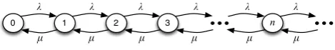
We first consider data traffic and assume that there is an infinite number of sources that are likely to generate traffic in the cell. We thus assume that requests for transmission globally arrive to the cell according to a Poisson process with rateλ. Each request brings an identically distributed volume of data to be transferred of meanxon. The

transmis-sion capacityCof the cell is equally shared among all active users, which is implemented by means of a Round-Robin dis-cipline. It is well-known that this system can be modeled by an M/M/1/∞/∞/Processor-Sharing (PS) queue with an ar-rival rateλand a service rateµ= C

xon. The straightforward

Markov chain associated with the PS queue is given in Fig-ure 1 (and is similar to that associated with a M/M/1/FIFO queue).

1

0 2 3

Figure 1: Markov chain associated with Scenario 1

If we denote byρ=λ

µ, it is widely known that the stability

condition of the queue isρ <1, and provided it is satisfied, the stationary probabilities of having n ongoing transmis-sions are given by:

p(n) = (1−ρ)ρn, n≥0 (1) Accordingly, the average number Q of active users in the system is:

Q=

∞

X

n=1

np(n) = ρ

1−ρ (2)

From Little’s law we obtain the average sojourn time of a user in the cell:

T = Q

λ =

1

µ−λ (3)

Finally, we can derive the average throughput obtained by users during their transfer in the cell (in bit/s) as:

γ= xon

T =C(1−ρ) (4)

2.2 Second scenario: data transmissions with

finite source (DF)

We still consider data traffic but we now assume that there is a finite number N of sources that are likely to generate traffic in the cell. Each one can be either idle or active, and generate traffic in the cell only when it is active. We still assume that the average data volume that any active user has to transferred is xon, and we denote bytof f the

aver-age time a user remains idle between two successive data transfers. The state of each user can thus be modeled as an ON-OFF process, and we assume that both the volume transferred during an ON period and the time spent during an OFF period are exponentially distributed (with respec-tive meansxon andtof f). This system can be modeled by

an M/M/1/N/N/P S queue with a service rate still given

byµ= C

xon and an arrival rateλ= 1

tof f. The Markov chain

(3)

( ) ( ) ( )

1

0 2 3

If we still defineρ= λ

µ, the queue length distribution is now

given by:

p(n) = N!

(N−n)!ρ

n

p(0), n= 0, ..., N (5)

withp(0) obtained by normalization. Note that there is no stability condition for this system (as it is actually a closed system). We can deduce the average number of active users in the cell:

Q=

N X

n=1

np(n) (6)

The average number of users that become active by unit of time is:

D=

N−1

X

n=0

p(n)(N−n)λ (7)

From Little’s law we obtain the average time a user stays active in the cell (between two successive idle times):

T = Q

D (8)

Finally, we can derive the average throughput obtained by users during their transfer as:

γ= xon

T (9)

2.3 Third scenario: voice transmissions with

infinite source (VI)

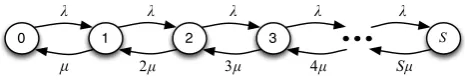
We now consider voice traffic and assume, like in the first scenario, an infinite number of sources. A voice transmission requires a throughput ofvbit/s. The total capacityCof the cell thus enables a maximum number of simultaneous voice calls given by:

S=bC

vc (10)

If we assume that requests for voice calls arrive according to a Poisson process with rateλ, and that call duration are exponentially distributed with rate µ = 1

ton (where ton is

the mean call duration), the system is modeled by a

classi-calM/M/S/S Markovian queue withS servers and a total

capacity limited toS. Figure 3 gives the associated Markov chain.

1

0 2 3

Still takingρ=λ_µ, the queue length distribution is given by the classical Erlang-B formula:

p(n) = ρ

n

n!p(0), n= 0, ..., S (11)

withp(0) obtained by normalization. Note again that there is no stability condition for this system (as it is limited). We can then calculate the average number of ongoing voice transmissions in the cell:

Q=

S X

n=1

np(n) (12)

Finally, PASTA property enables us to derive the rejection probability of a call request:

Pr=p(S) (13)

2.4 Fourth scenario: voice transmissions with

finite source (VF)

We finally consider voice traffic and assume, like in the sec-ond scenario, a finite numberNof sources. Each source fol-lows an ON-OFF process, an ON corresponding to a voice call and an OFF corresponding to the idle time between two successive calls. We assume that both the time spent dur-ing an ON period and the time spent durdur-ing an OFF period are exponentially distributed, with respective meanstonand

tof f. We define the arrival rateλ= _t1

of f and the service rate

µ= 1

ton.

We need to distinguish two cases: 1) N ≤ S, in which case the capacity of the cell is enough to serve all the N

users simultaneously. As a result, no call rejection can oc-cur; 2)N > S, in which case the capacity of the cell is not enough to serve all users simultaneously, and call rejections can happen. Markov chains associated with the two cases are given in Figure 4. In both cases there is no stability condition for the system.

( ) ( ) ( )

( ) ( ) ( ) ( + )

1

0 2 3

1

0 2 3

Figure 4: Markov chains associated with Scenario 4 (up: N≤S, down: N > S)

For the first case,N ≤S, the queue length distribution is:

p(n) = N!

n!(N−n)!ρ

n

p(0), n= 0, ..., N (14)

withρ= λ_µ andp(0) obtained by normalization. The aver-age number of active users in the cell is:

Q=

N X

n=1

np(n) (15)

And as the capacity of the cell is enough to serve all users simultaneously, there is no possible rejection (the rejection probability is null).

(4)

are limited ton=S:

p(n) = N!

n!(N−n)!ρ

n

p(0), n= 0, ..., S (16)

withp(0) obtained by normalization. The average number of active users in the cell is now:

Q=

S X

n=1

np(n) (17)

And the rejection probability can be expressed as the fol-lowing rate ratio:

Pr =

p(S)(N−S)λ

S X

n=0

p(n)(N−n)λ

(18)

3. VIENNA AND NS-3 LTE SIMULATORS

We present in this section the main characteristics of the two simulators we compare on the four scenarios of Section 2.

3.1 Vienna Simulator

The Vienna LTE System Level Simulator was created by the Institute of Telecommunications at the Vienna University of Technology. It is an open source software developed in MAT-LAB using the Object-Oriented programming (OOP) capa-bilities that have been introduced with the release 2008a. The simulator is available from [10]. The project first devel-oped a link level simulator before extending it to a system level simulator. While link-level simulations allow for the research on issues such as Multiple Input Multiple Output (MIMO) gains, Adaptive Modulation and Coding (AMC) feedback, modeling of channel encoding and decoding, sys-tem level simulations is more dedicated to network-related issues such as scheduling, mobility handling, interference management or signals propagation [11]. In system level simulations, the physical layer is abstracted from link level results and used for evaluating network performance. The system level simulator follows the structure shown in Fig-ure 5. Each network element is represented by a suitable MATLAB class object.

The network topology is created as follows: a specific region of interest (ROI) is generated and divided into transmission sites or cells, to each one an eNodeB is appended. Each eN-odeB contains a scheduler (see Figure 5). After creating the topology, one or many User Equipments (UEs) are deployed according to a specific spatial distribution model (only a con-stant number of users per cell with random positions is sup-ported). Users can be either fixed or mobile (with a specific mobility model). Once the network created, the Vienna sim-ulation main loop is carried out for each Transmission Time Interval (TTI) of 1ms: Depending on the scheduling algo-rithm and the received UEs feedbacks the scheduler assigns Resource Blocks (RBs) and a MCS to each UE attached to an eNodeB. At the UE side, the Signal-to-Interference and Noise Ratio (SINR) is calculated per received subcarrier. At the end of each time-step, link performance measurements are performed to provide the simulation output which con-sists of traces, containing link throughput and error ratios for each user, as well as summary measures by cell, from which statistical distributions of throughputs and errors can be extracted.

scheduler RB allocation

channel adaptation (MCS assignment) eNodeB

macroscopic pathloss shadow fading

fast fading UE-specific signaling

downlink channels

UEs

subcarrier SINR calculation

SINR-to-CQI mapping

SINR-to-BLER mapping

feedback uplink channel feedback uplink

channel feedback uplink

channel

BLER, throughput traffic

model calcula mobility

model calculati

sig

n

al

in

te

rferenc

e

noise signaling

Figure 5: Block diagram of the LTE system level simulator [11]

The simulator contains a main MATLAB fileLTE sim main.m which executes the pseudo-code below:

create the network

foreach simulated TTIdo if mobile UEsthen move UEs

if UE outside ROIthen reallocate UE randomly in ROI foreach eNodeBdo

receive UE feedback after a given feedback delay schedule users

foreach UEdo

1- channel state→link quality measurements→SINR 2- SINR, MCS→link performance measurements→BLER 3- send UE feedback

For running the simulation, one has to write a MATLAB script which must perform the following tasks:

• Either loading a configuration file (in the +simula-tion config subfolder) which applies a specific pre-configured simulation parameters, or configuring the parameters manually.

• Executing the main simulation file.

3.2 NS-3 Simulator

(5)

NS-3 was developed using the C++ programming language and is a free simulator under GPLv2 License. It can be downloaded from the ns-3 webpage [13], where a manual and tutorials can also be found. We used for this comparison the ns-3.20 version. Figure 6 shows the hierarchy of the ns-3 classes.

Figure 6: Software organization of the ns-3 simula-tor [13]

In ns-3 one has to write a script in C++ (or Python) with the include files, the topology of the network, the rout-ing, the tracing and the applications. This script is run using a waf command: waf --run myProgram --command-template="%s --RngRun=2", where “RngRun” gives the sim-ulation run number. In order to compute statistics using independent runs one has to set a different number for each run.

4. SIMULATOR COMPARISON

In this section, we compare the easiness to simulate on both tools the four scenarios described in Section 2, and analyze their accuracy in terms of run-time duration and memory and CPU usage.

4.1 Generalities

As detailed in Section 2, for comparing the two simulators we defined four simple scenarios1_{: (DI) data traffic with}

in-finite source, (DF) data traffic with in-finite source, (VI) voice traffic with infinite source, and (VF) voice traffic with finite source. The comparison is essentially carried out with re-spect to accuracy. However, for the most loaded scenario we also compare memory usage, computation time and CPU utilization. We also want to give a glimpse on their ease of handling, the realism of modeling assumptions and the ease of obtaining performance from traces of simulation.

The main differences between these two simulators are:

• NS-3 is a general network simulator that can be used to simulate many protocols and technologies, not only LTE. Instead Vienna is a specialized LTE simulator.

• Vienna advances the time by time-slices (of 1ms), while ns-3 does by the date of the next event: ns-3 is a dis-crete event simulator.

1

all code are available upon demand to authors

• Vienna is very precise on the modeling of the physical layer. At each TTI it performs many calculations at the physical layer level. These computations drasti-cally slowdown the simulation which may make unfea-sible the simulation of more realistic scenarios. On the other hand,ns-3 uses a correspondence table provided by the 3GPP LTE specifications, that directly links a certain MCS, the number of RBs the antennas are us-ing and the transport block (TB) size [14]. Therefore, at each transmission, the simulator just retrieves such information, instead of calculating them, which results in an substantial gain.

• The code organization in ns-3 is very clear: each tech-nology has a separate module and each class corre-sponds to a network real object. In Vienna modularity is not well exploited and it is not easy to create new classes without modifying many other files.

• Traces provided by Vienna are simple to treat and one can also easily add other type of traces if needed. In ns-3 traces collection and processing is cumbersome.

In order to perform the simulation of our four basic scenar-ios, we had to overcome some intrinsic limitations of the two simulators:

• Due to its lack of modularity, it is very complicated to make any code modifications in Vienna. The solution we found to improve the speed of the simulator was to perform the physical layer calculations only when an UE perceives a change in channel conditions, instead of doing them at each TTI.

• Vienna requires a constant number of users deployed per cell. For the DI and VI scenarios, where the total number of UEs in the cell varies with time, we had to make changes in the code of the simulator in order to allow the creation of new users on-the-fly. From the ns-3 side, the simulator limits to 320 the number of nodes to be created and connected to an eNodeB. We thus have to re-use nodes after a certain time of inactivity for overcoming such limitation.

• To simulate the DF scenario, we had to implement the ON-OFF traffic as a new application in both simula-tors. Indeed, such a traffic with an ON period charac-terized by a downloaded size (instead of a time) was not part of existing modules.

• For the voice cases (VF and VI) we had to implement a new scheduler policy in order to take into account rejection.

(6)

time-step to store the IDs of rejected UEs if a rejection takes place. At each time-step event and following theblocked ids values, theblocked parameter, which we have created as at-tribute of each UE, takes“true” if he is rejected and “false” in the other case. An output vector,rejected, with total TTIs as length has been added to theUEs traces.matoutput trace file. This vector stores for each UE all the values taken by theblockedattribute from which we can extract the number of times that an UE was rejected.

In ns-3, we used the trace files to derive the performance measures. Among the files, the DLPdcpStats.txt provides for each TTI the amount of data downloaded by the active users. We filtered that file to extract the mean ON and OFF periods of each user, their average throughput and the mean number of active users. Moreover, we added to the system output the ability of identifying all rejections of UE’s, when-ever they take place. By combining the number of times a rejection occur for an UE with the statistics obtained from the DLPdcpStats.txt file, we obtained the rejection proba-bilities of the system.

4.2 DI: data traffic with infinite source

For this scenario we implement the mechanisms described in Section 2.1. In our simulation the transmission ends when the corresponding user completes the download of an expo-nentially distributed amount of data with mean xon. We

assume that new data transfers arrive according to a Pois-son process, meaning that the time between two successive arrivals is exponentially distributed with meantof f = 1λ.

As aforementioned, the Vienna simulator did not address this “open” case (where new UE demands arrive from the outside according to a Poisson process). We thus modified the simulator in order to be able to add, remove and reuse UEs during the simulation.

In order to simulate this scenario with ns-3, we came across a problem: the number of nodes (UEs that request service) that can be created is limited to 320. This limitation is due to LTE specifications. Therefore, instead of creating a node for each new arrival, we reused those already created and served. But this forced us to create a mechanism for differentiating the reused nodes in the traces.

In both simulators we consider a Single Input Single Output (SISO) single cell of diameter 500 meters. 10 UEs are static in the cell and make data transfers with mean parameters

xon= 1.7Mbits andtof f (the inter-arrivals time) mean

dis-tribution varied from 100ms to 150ms. We have configured the system bandwidth to 5MHz which is equivalent to 25 RBs. For the link quality measurements we used a simple channel model with only path-loss supported. The transmis-sion power has been set to 1wattswhich allow all users to give the same and best MCS anywhere in the cell. With 25 RBs and for the best given MCS, we obtain a cell capacity

C of 18336 bits/ms (according to the technical specifica-tions described in [14]). Each simulation was executed 300 seconds.

For this scenario the simulated parameters are in Table 1. Each simulation has been executed 10 times and 95% confi-dence intervals were computed.

System frequency 2.6GHz

System bandwidth 5MHz (25 RBs)

Channel model Only pathloss supported with the Free space model

Diameter of the cell 500m

Transmission power 1W (best MCS in the cell)

Transmission mode SISO

Scheduler Round Robin

Mean sizexon 1.7Mbits

Mean inter-arrival timetof f from 100ms to 150ms

Simulation time 300s

Table 1: Simulation parameters of the DI model

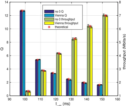
Figure 7 depicts a performance comparison on the accuracy between the two simulators and the theoretical model in terms of the mean number of active users (eq. (2)) and the average throughput (eq. (4)).

t o f f (ms)

90 100 110 120 130 140 150 160

Q

0 2 4 6 8 10 12 14

throughput (Mbits/s)

1 2 3 4 5 6 7 8

ns-3 Q Vienna Q ns-3 throughput Vienna throughput theoretical

Figure 7: Average number of active users (Q) and mean throughput for the DI scenario.

One can see from this figure that both simulators are ac-curate. But ns-3 seems more accurate with a relative error (Er) less than 0,5% (i.e.,Er<0,005) while Vienna shows a

Er inferior than 3,9% for the mean number of active users.

For the mean throughput ns-3 still having the same relative error and Vienna has a Er less than 2,5%. Note however

that in all cases the theoretical values are covered by the confidence intervals.

4.3 DF: data traffic with finite source

(7)

The two parameters that change with respect to the DI sce-nario are depicted in Table 2.

Number of users in the cell 10

Mean OFF periodtof f from 200ms to 1200ms

Table 2: Simulation parameters of the DF model

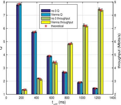
Figure 8 compares the average number of active users (eq. (6)) as well as the mean throughput (eq. (9)) for a varyingtof f.

t_{of f} (ms)

0 200 400 600 800 1000 1200 1400

Q

1 2 3 4 5 6 7 8

throughput (Mbits/s)

2 3 4 5 6 7 8 9

ns-3 Q Vienna Q ns-3 throughput Vienna throughput theoretical

Figure 8: Average number of active users (Q) and mean throughput for the DF scenario.

Results reveal again no significant errors between simulation and analysis. In this case, Vienna provides a better accuracy on parameterQthan ns-3, with aErof 0.7% instead of 1.9%.

Concerning the mean throughput, theEr provided by

ns-3 is of almost 1% while Vienna has aEr of around 1.9%.

Moreover, we observe that the 95% confidence intervals are quite narrow and include the true values in all cases for both simulators.

4.4 VI: voice traffic with infinite source

As explained in Section 2, the main difference between data traffic and voice traffic resides in the fact that ON periods are not characterized anymore by a size (of downloaded el-ements), but instead by a time (of conversations). We thus characterize the activity session by an exponential distribu-tion of meanton.

As in this scenario the number of sources is infinite, we reuse the procedure for creating users, as explained in the DI sce-nario. We assume that new call demands arrive according to a Poisson process, meaning that the time between two successive arrivals is exponentially distributed with mean

tof f =_λ1.

For the VI scenario we simulate a single cell with the pa-rameters listed in Table 3. We are aware thatton andtof f

of the order of hundred of milliseconds do not correspond to reality. But based on theoretical results, we know that the

performance parameters of the system is only sensitive to the ratio ofton andtof f. Consequently we chose small

val-ues in order to significantly reduce the simulation run-times. This is even more important in the case of Vienna simulator that runs at a TTI time-step.

Scheduler Round Robin (modified to reject calls)

Number of servers 10

Mean ON periodton 1000ms

Table 3: Simulation parameters of the VI model

Figure 9 compares simulation results with analytical values, for both performance parameters of interest, the average number of active usersQ(eq. (12)) and the rejection prob-ability Pr (eq. (13)). It shows that ns-3 yields little more

precise estimation than Vienna. The relative error on Qis less than 0,38% for ns-3 and less than 0,59% for Vienna. Concerning Pr errors are inferior to 0,36% and 4,86% for

ns-3 and Vienna respectively. Despite this difference, we can say that both simulators produce comparable results, as in both cases the 95% confidence intervals always contain the actual values and no significant deviation between the exact and the simulated statistics is observed.

t of f (ms)

90 100 110 120 130 140 150 160

Q

6 6.5 7 7.5 8

Pr

0.05 0.1 0.15 0.2 0.25

ns-3 Q Vienna Q ns-3 Pr Vienna Pr theoretical

Figure 9: Average number of active users (Q) and rejecting calls probability (Pr) for the VI scenario.

4.5 VF voice traffic with finite source

For this scenario we configured our two simulation scripts to model a single-cell system with a constant numberN = 15 of users that perform an ON-OFF traffic with aton= 950ms

for the exponential distribution. We varytof f from 200ms

(8)

diameter 500 meters. The parameters are summarized in Table 4.

Scheduler Round Robin (modified to reject calls)

Number of servers 10,20

Number of users 15

Mean ON periodton 950ms

Table 4: Simulation parameters of the VF model

The average number of active usersQ(eq. (17)) as well as the probability of rejecting a callPr(eq. (18)) are compared

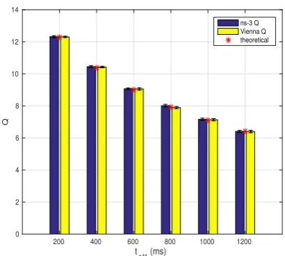
in Figure 10 for the case whereN > S. Figure 11 only gives

Qin the case where theN≤S(as in this case the rejection probability is null, see eq. (15)). The 95% confidence inter-vals estimated from a sample of 10 replications are indicated for each value.

t_{o f f} (ms)

0 200 400 600 800 1000 1200 1400

Q

6.5 7 7.5 8 8.5 9 9.5 10

Pr

0 0.1 0.2 0.3 0.4 0.5 0.6 0.7 ns-3 Q Vienna Q ns-3 Pr Vienna Pr theoretical

Figure 10: Average number of active users (Q) and rejecting calls probability (Pr) for the N > S VF.

Again, the results of both simulators match exact results with a pretty good accuracy. In the first case (N > S), relative errors for Q are smaller than 0,59% for ns-3 and less than 0,83% for Vienna. ConcerningPr, the difference

remains small for ns-3, less than 0,58%, but becomes bigger for Vienna, around 9,5%. In the second case (N ≤S), the relative errors onQremain inferior to 0,9% for ns-3 and to 0,64% for Vienna. In this case, Vienna is thus slightly more accurate than ns-3.

4.6 Performance comparison

In order to compare the simulation run-time, memory usage and CPU occupation we conducted simulations on a 8 cores Intel(R) Xeon(R) CPU E5-2450 v2 @ 2.50GHz workstation with 64GB of RAM, running Ubuntu Linux 14.04 LTS.

t o f f (ms)

200 400 600 800 1000 1200

Q

0 2 4 6 8 10 12 14

ns-3 Q Vienna Q theoretical

Figure 11: Average number of active users (Q) for the N≤S VF.

Tables 5, 6 and 7 show the different measured performance metrics for each simulator. These results correspond to the simulation of the most loaded scenario.

In both ns-3 and Vienna, the run-time performance is di-rectly provided as an output of our scripts. For the mea-surement of the memory and CPU occupation performance, we used thetopprogram of Linux which provides a dynamic real-time view of the system: when a simulation is running, we periodically observed the used amount of memory and the CPU utilization and the final results were averaged over the number of observations.

model VF DF VI DI

ns-3 37min 27min 465min 608min Vienna 780min 390min 270min 300min

Table 5: Comparison of the run-time

(9)

computation time than Vienna. This difference is due to the fact that the two simulators use different networks with different scales to carry out infinite source simulations. In-deed, ns-3 models the infinite source by a large number of UEs per cell (320 nodes) while in Vienna we can create and eliminate nodes at runtime.

model VF DF VI DI

ns-3 52MB 44MB 71MB 64MB

Vienna 1.6GB 1.25GB 2.25GB 3GB

Table 6: Comparison of the memory usage

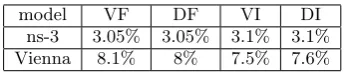
model VF DF VI DI

ns-3 3.05% 3.05% 3.1% 3.1%

Vienna 8.1% 8% 7.5% 7.6%

Table 7: Comparison of the CPU occupation

Regarding the memory we can clearly see the superiority of ns-3 over Vienna which uses as much as 46 times more memory. We saw a big difference in memory between infinite and finite source scenarios.

For CPU utilization, ns-3 uses less resources than Vienna but the difference is not as high as for memory.

5. CONCLUSIONS

We have compared two simulators, ns-3 and Vienna, in the context of LTE networks, on four basic scenarios for which well-known analytical results exist. We evaluated both of them in terms of accuracy, ease of handling and use, execu-tion time, memory and CPU usage. Our conclusions are the following:

First, in terms of accuracy, both simulators provide good results. Both give small errors when compared to theoretical values and narrow confidence intervals for the four scenarios we tested.

Second, regarding the execution time, there are important differences between simulators. For the scenarios with a fi-nite number of sources, ns-3 is clearly faster than Vienna. However, Vienna becomes faster for infinite source scenar-ios. This can be explained by the fact that in ns-3 we need to create at the beginning of the simulation a fixed and suf-ficiently big number of UEs, whereas in Vienna, UEs can be created and deleted on-the-fly.

Third, in terms of CPU and memory usage, ns-3 is much better than Vienna. While ns-3 is based on C++, Vienna is based on the MATLAB environment, which requires enor-mous amounts of memory to run.

Fourth, concerning the ease of handling and use, the choice is somehow subjective, it depends on the skills of the pro-grammer, in C++ or in MATLAB language. However, we find that output traces are easier to manipulate in Vienna than in ns-3. In the other hand, ns-3 is quite well docu-mented which is not the case for Vienna.

Finally, taking into account the four aforementioned points and the experience acquired with this simulation compar-ison, we believe that ns-3 is a better choice for simulat-ing more complex scenarios, includsimulat-ing different codsimulat-ing zones within the cell, different cells, inter-cell traffic and UE’s mo-bility. These more complex scenarios correspond to the re-cent work we are carrying out in the framework of the IDE-FIX project.

Acknowledgment

This work has been carried out in the framework of IDE-FIX project, funded by the ANR under the contract number ANR-13-INFR-0006.

6. REFERENCES

[1] E. Dahlman, S. Parkvall, J. Skold, and P. Beming.3G Evolution: HSDPA and LTE for Mobile Broadband. Academic Press, 2th edition, 2007.

[2] Intelligent design of future mobile internet for enhanced experience. http://lia.univ-avignon.fr/idefix/.

[3] E. Weingartner, H. vom Lehn, and K. Wehrle. A performance comparison of recent network simulators. In IEEE International Conference on Communications (ICC), pages 1–5, June 2009.

[4] A.R. Khan, S.M. Bilal, and M. Othman. A performance comparison of open source network simulators for wireless networks. InIEEE International Conference on Control System, Computing and Engineering (ICCSCE), pages 34–38, Nov 2012.

[5] M. H. Kabir, S. Islam, Md. J. Hossain, and S. Hossain. Detail comparison of network simulators.International Journal of Scientific & Engineering Research, 5:203–218, october 2014.

[6] E. Schoch, M. Feiri, F. Kargl, and M. Weber. Simulation of ad hoc networks: ns-2 compared to JiST/SWANS. InICST International Conference on Simulation Tools and Techniques for Communications, Networks and Systems & Workshops (SIMUTools), pages 36–43, march 2008. [7] G. F. Lucio, M. Paredes-Farrera, E. Jammeh, M. Fleury,

and M. J. Reed. Opnet modeler and ns-2: Comparing the accuracy of network simulators for packet-level analysis using a network testbed. InWEAS International Conference on Simulation, Modelling and Optimization (ICOSMO), pages 700–707, october 2003.

[8] E. Altman and T. Jimenez.NS Simulator for Beginners. Synthesis Lectures on Communication Networks. Morgan, 2012.

[9] L. Kleinrock.Queueing Systems, Volume 1: Theory. Wiley-Interscience, 1975.

[10] LTE simulators.

http://www.nt.tuwien.ac.at/research/mobile-communications/vienna-lte-a-simulators/.

[11] J. C. Ikuno, M. Wrulich, and M. Rupp. System level simulation of LTE networks. InIEEE Vehicular Technology Conference (VTC), pages 1–5, May 2010.

[12] The LENA Project. http://networks.cttc.es/mobile-networks/software-tools/ns-3/.

[13] NS3 network simulator. http://www.nsnam.org/. [14] European Telecommunications Standards Institute. LTE;

Comparative study of LTE simulations with the ns-3 and the Vienna simulators