Intelligent Contextual Algorithm For Harmonics Classification

Intelligent Contextual Algorithm For

Harmonics Classification

1_{M.K. ELANGO}

Professor,Department of EEE, K.S.Rangasamy college of technology, Tiruchengode, Namakkal (Dt), Tamil nadu, India-637215

2 _{Dr. A. NIRMAL KUMAR}

Professor, Department of EEE, Info Institute of Engineering, Kovilpalayam, Coimbatore, Tamil Nadu, India, -641107

1 _{Email: [email protected]. Fax: 04288-274745. Mobile: 00-91-9952493666.} 2 _{Email: [email protected]. Fax: 0422-2654888. Mobile: 00-91-9842524957.}

Abstract:

This paper presents methods for classification of harmonics present in the electrical signal using Fast Fourier Transform (FFT), Contextual Clustering (CC) and Back Propagation Algorithm (BPA). Power quality meter has been used to collect the electrical signal data from a 40W Fluorescent Lamp (FL). In the captured data, various electrical disturbances are introduced through Matlab code. FFT has been used for extraction of features from the acquired electrical signal. The FFT, CC, BPA and BPACC algorithms have been implemented by Matlab. Comparison of performance classification of harmonics by CC, BPA and BPACC are presented.

Keywords: Contextual Clustering, Back Propagation Algorithm, Harmonics, Power Quality, Fast Fourier Transform.

1. Introduction

 The life of electrical equipment is based on the quality of the electrical signals that form the inputs for the electrical equipments. Repeated power cuts, spikes, sags, swells and other disturbances in the power lines will lead to different orders of harmonics in the electrical signal and hence the life of the electrical equipment is reduced. The concept of power quality of the electrical signal will decide the life of equipments. There is urgency for developing novel algorithms that can classify the type of harmonics and other electrical disturbances. Many algorithms have been developed by the researchers for classification of electrical disturbances. Some of them are S-Transform and two dimensional time–time (TT) transform [Suja and Jovitha, (2010)], Integrated Fourier linear combiner and fuzzy expert system [Dash et al (1999)], multiwavelet-based neural networks [Suriya et al (2008), Murat et al (2008),

Mário et al (2009)], least absolute value (LAV) state estimation algorithm to measure the flicker voltage magnitude

[Soliman and El-Hawary (2000)], simulated annealing [Solimana et al (2004)], fast fourier transform and neural

network [Dash et al (1998)], fuzzy estimation of voltage flicker[Bhim Singh et al (1999) ], Chirp-Z transform

(CZT) [Aiello. et al (2005)], Adaptative Kalman filtering [Pradhan et al (2004)], short-time Fourier Transform

[Leonowicz et al (2003)], least-squares sine-fitting [Fonseca et al (2004)],hidden Markov model [Brown et al

(1996)], template matching [Elmitwally et al (2000)] and rule based system [Zheng et al (2002)].

such as the time-scale, frequency or amplitude of the signal. The hidden Markov model can overcome the changes in the basic scale changes.

In this work, we propose and improved contextual clustering [Eero et al (2001)] and supervised back

propagation neural network algorithm for electrical disturbance classification. These two algorithms use the frequency domain features extracted using FFT technique.

2. Materials and Methods

2.1 Schematic diagram

Schematic diagrams of training and testing of the proposed algorithms are shown in figure 1 and figure 2  respectively

Fig.1 Training the proposed algorithm

Fig.2 Testing the proposed algorithm

Figure 1 and Figure 2 show the sequence of blocks for extracting features of the electrical signal from the 40W FL and the method of training the CC and the BPA. In general electrical signal is acquired from the power line and used as input for the analog to digital converter (ADC). The FFT algorithm is used to convert the time domain signal information into a frequency domain information. The different frequencies, their power of magnitude, phase angles are calculated and they are given as inputs for contextual clustering and back propagation algorithm for training purpose. At the end of training, the learned information in the form of weights is stored as weight database. During, the actual implementation of classification of electrical disturbances, the weight database is provided with the features extracted from the ADC signal. Based on the classified information, subsequent triggering of hardware is done.

2.2 Contextual clustering

Contextual segmentation refers to the process of partitioning a data into multiple regions. The goal of segmentation is to simplify and / or change the representation of data into something that is more meaningful and easier to analyze. Data segmentation is typically used to locate data in a vector. The result of contextual segmentation is a set of regions that collectively cover the entire data. Each value in a data is similar with respect to some characteristic.

Power line   ADC  

Frequency, magnitude, phase

Proposed algorithms

Trained database

Power line   ADC  

Frequency, magnitude,  phase

Process with the database

Identify the disturbances

Adjacent regions are significantly different with respect to the same characteristics. Contextual clustering algorithms which segments a data into one category (ω0) and another category (ω1). The data of the background are assumed to be drawn from standard normal distribution.

1. Define decision parameter Tcc (positive) and weight of neighbourhood information β (positive). Let Nn be the total number of data in the neighbourhood. Let Zi be the data.

2. Initialization: classify element of data with Zi>Tcc to ω1 and element of data to ω0. Store the classification to C0 and C1.

3. For each element of data ‘i’, count the number of data ui, belonging to class ω1 in the neighbourhood of data ‘i’. Assume that the element of data outside the data area belong to ω0.

4. Classify element of data with _i n _α

cc

i

₂

)

T

N

(u

T

β

z







5. If C2 ≠C1 and C2 ≠ C0, copy C1 to C0, C2 to C1 and return to step 3, otherwise stop and return to C2.

2.3 Back Propagation Algorithm

Artificial Neural Network is the simulation of human brain. It has been modeled to map inputs with target outputs. Back propagation algorithm is a supervised method which maps the features of an electrical signal to a predefined classification category of electrical disturbances. The BPA learns the features using the steepest decent concept.

Input Hidden Output layer layer layer

Fig.3 Multilayer Perceptron

Figure 3 shows the topology of ANN trained by using BPA. Information flow from input layer to output layer through hidden layer. Learning is done by updating weights from output layer to input layer through hidden layer. The training is stopped one the desired mean squared error (MSE) is reached.

3. Experimental Method

Fig.4 Measurement of Electrical signal using Fluke meter

0 100 200 300 400 500 600 700 800 900 1000

-250 -200 -150 -100 -50 0 50 100 150 200 250

Time, ms

A

m

pli

tude

, V

o

lt

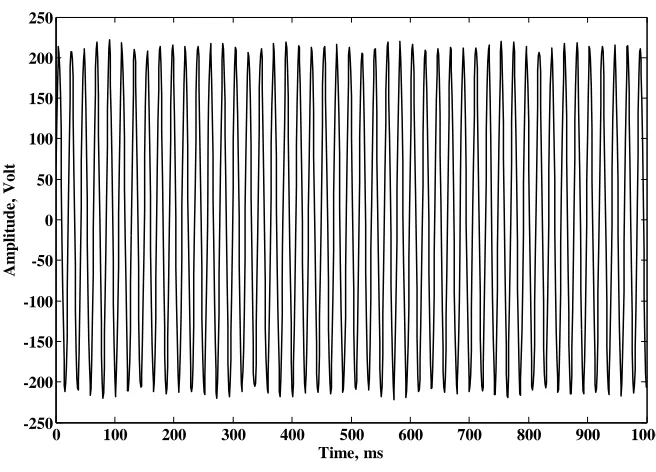
Fig. 5 Wave form for the 40 Watts FL

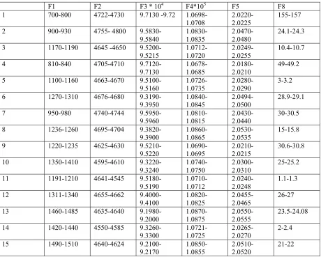
Table 1 gives the details of frequency, phase voltage values for all the screen shots of fluke meter.

Table 1 Parameter values for the fluke meter output

frequency, f=[46.76 97.56 146.3 195.1 244.1 293 0] phase,



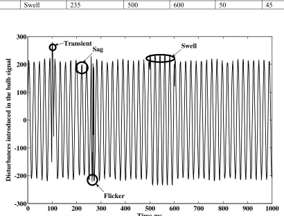
Table 2 shows various values of voltage amplitude, starting and ending time of the disturbances, frequency and phase angle for each disturbance. A sample of electrical disturbance waveform which is a combination of values given in 14th _{row of Table 3 is presented in Figure 6.}

Table 2 Disturbances used for creating additional wave details

S.No Type Amplitude, Volts Time start, ms

Time End, ms

Frequency Phase

1 Pure sine

wave 230 0 1000 50 0

2 Transient 280 100 105 50 20

3 Sag 200 200 250 50 45

4 Flicker 1 238 260 262 204 45

5 Flicker 2 222 263 265 159 45

6 Flicker 3 238 266 268 250 45

7 Flicker 4 222 269 271 200 45

8 Swell 235 500 600 50 45

0 100 200 300 400 500 600 700 800 900 1000

-300 -200 -100 0 100 200 300

Time,ms

D

is

tur

b

a

nc

e

s intr

o

duc

e

d

i

n

th

e

bulb

si

g

n

a

l

Transient Sag

Flicker

Swell

Fig. 6 Plot of FL signal with electrical disturbances

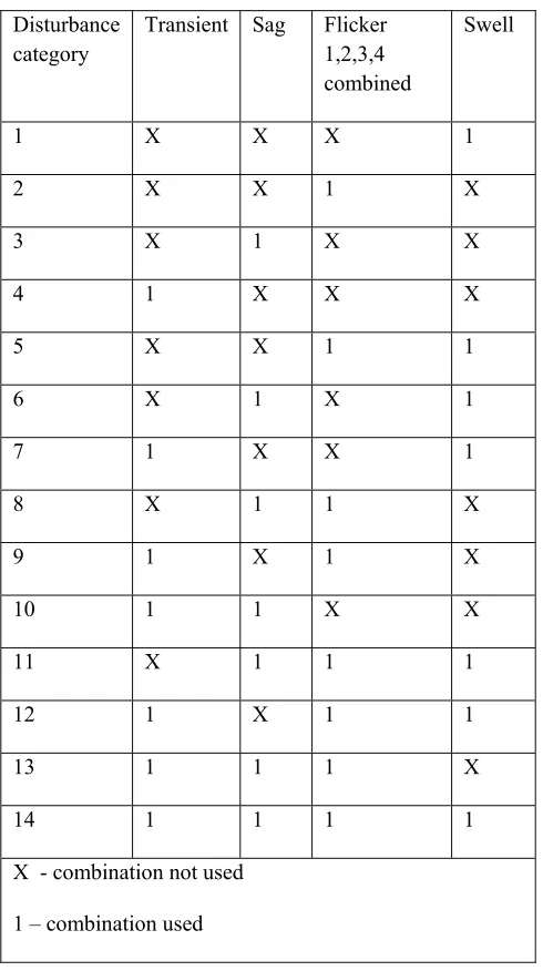
Table 3 Waveform generation with different combinations of electrical disturbances

Disturbance category

Transient Sag Flicker 1,2,3,4 combined

Swell

1 X X X 1

2 X X 1 X

3 X 1 X X

4 1 X X X

5 X X 1 1

6 X 1 X 1

7 1 X X 1

8 X 1 1 X

9 1 X 1 X

10 1 1 X X

11 X 1 1 1

12 1 X 1 1

13 1 1 1 X

14 1 1 1 1

X - combination not used 1 – combination used  

4. Feature Extraction

The time domain electrical signal is obtained using FFT. The signal has been sampled at 1000Hz as the maximum harmonic frequency that will be identified in the electrical signal is 500Hz.

n 1 i

(i))

+

t

*

f(i)

*

*

sin(2

*

v(i)

+

s

=

s





z=FFT(s) = x+ jy (2)

where

z is the complex representation of the time sampled signal transformed in the frequency domain using FFT x is the real component of the complex number

y is the imaginary component of the complex number j is imaginary part

n is order of harmonics

Pm= (x2 _{+ y}2₎1/2 ₍₃₎

Pm is the power of magnitude

Mean of power of magnitude

F1=

p

(i)

n

1

1

i m





(4)

Standard deviation of real component

F2=

(P

(i)

P

(i)

)

n

1

m F

1

i m

s







(5)

Maximum power of magnitude

F3=max(Pm) (6)

Norm of the signal

F4=

s m

F

P

(7)

Total harmonic distortion

F5= ₂

f Fs

1 i

2 m

V

(i)

)

(P





Vh

(8)

where

Vf is the voltage corresponding to fundamental frequency (230v at 50 Hz)

(P

)

Minimum frequency in the signal with and without disturbances

F6=min(fh) (9)

Maximum frequency in the signal with and without disturbances

Minimum power of magnitude in the signal with and without disturbances

F8=

min((P

)

)

Maximum power of magnitude in the signal with and without disturbances

F9=

max((P

)

)

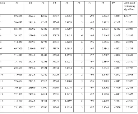
Table 4 presents the feature values extracted for 15 combination of signal generated. Here, the feature of the original signal is also presented with 14 combination. Hence, we have 15 rows when compared to that of 14 rows in Table 3.

Table 4 Features of the wave form with different disturbances

S.No F1 F2 F3 F4 F5 F6 F7 F8 F9 Label used

for training algorithms

1 69.2688 2123.3 13862 47457 0.8963 48 293 0.3333 42854 1.7919

2 70.6233 2361.0 45323 52765 0.9974 3 497 0.4952 45323 2.1876

3 68.4354 2179.2 42402 48703 0.9207 3 496 2.3035 42402 2.1008

4 70.1002 2280.9 45973 50975 0.9635 6 496 0.0665 45973 2.1887

5 71.8350 2189.3 42794 48931 0.9250 6 496 0.1646 42794 2.1072

6 69.7900 2.410.9 44871 53879 1.0185 3 497 0.9842 44871 2.1743

7 71.4547 2504.1 48442 55960 1.0578 3 497 0.7007 48442 2.2607

8 73.1895 2421.8 45263 54124 1.0231 3 497 0.6849 45263 2.1810

9 69.2669 2332.6 45521 52130 0.9854 2 496 0.1045 45521 2.1756

10 71.0016 2242.6 42342 50120 0.9475 2 496 1.8493 42342 2.0948

11 72.6664 2343.2 45913 52369 0.9900 5 496 0.0989 45913 2.1820

12 70.6214 2550.9 47990 57005 1.0776 3 497 3.4702 47990 2.2468

13 72.3562 2469.6 44811 55191 1.0433 3 497 1.6990 44811 2.1673

14 71.8330 2392.8 45461 53476 1.0109 5 496 0.2980 45461 2.1687

5. Results and Discussions

5.1 Output of Contextual clustering

0 1 2 3 4 5 6 7 8 9 10 11 12 13 14 1515

1.7 1.8 1.9 2 2.1 2.2 2.3 2.4 2.5 2.6

Electrical disturbances

E

sti

ma

te

d a

n

d ta

r

g

e

t o

utp

uts

Target

CC output

Fig.7 Performance of contextual clustering

The Figure 7 shows the plot of estimation of contextual clustering. The values have been plotted against the target values. The target values are the average of the feature values for each disturbance. During averaging, the feature values are normalized to the first decimal. During training of the contextual clustering, no target value is used. Training is based on the neighboring values of the features in each wave form.

5.2 Outputs of Back propagation algorithm

0 500 1000 1500 2000

-0.15 -0.1 -0.05 0 0.05 0.1 0.15

Iterations

MS

E

9 X 2 X 1

Fig.8 MSE curve during learning phase of BPA

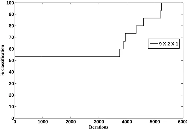
number of nodes in the output layer is 1. The Figure 9 presents the classification performance of the BPA for every iteration. The classification performance is calculated as the number of test patterns are correctly classified with respect to total number of test patterns in each iteration. The classification performance remains about 50% during the first 3800 iterations and there is continuous improvement of classification performance after 3800 iterations. 100% classification performance is achieved after 5000 iterations. Figure 10 shows the actual target output (solid line) used for training the BPA and the estimated output obtained during testing (dotted line).

0 1000 2000 3000 4000 5000 6000

0 10 20 30 40 50 60 70 80 90 100

Iterations

%

c

las

si

fi

c

at

ion

9 X 2 X 1

Fig. 9 Learning performance of BPA for all the training and testing patterns

1 2 3 4 5 6 7 8 9 10 11 12 13 14 1515

1.7 1.8 1.9 2 2.1 2.2 2.3 2.4

Electrical disturbances

E

sti

ma

te

d

a

n

d

ta

r

g

e

t o

u

tpu

ts

Target BPA output

Fig. 10 Performance of BPA

5.3 Classification of The Electrical Disturbances Using The Feature Values

If (F1<=800 and F1 >=700) and (F2>=4722 and F2<=4730)

and (F3<=9.72*10e03 and F3>=9.713*10e03) and (F4<=1.0708*10e05 and F4>=1.0698*10e05) and (F5<=2.0225 and F5>=2.022)

and (F8<=157 and F8>=155) then display(‘Type 1 signal’) end

The above procedure is repeated for all 15 signals mentioned with various electrical disturbances.

Table 5 Classification of the electrical disturbances using template matching

F1 F2 F3 * 104 _F4*105 _{F5 F8}

1 700-800 4722-4730 9.7130 -9.72

1.0698-1.0708 2.0220-2.0225 155-157

2 900-930 4755- 4800

9.5830-9.5840 1.0830- 1.0835 2.0470-2.0480 24.1-24.3 3 1170-1190 4645 -4650

9.5200-9.5215

1.0712- 1.0720

2.0249-2.0255

10.4-10.7

4 810-840 4705-4710

9.7120-9.7130 1.0678- 1.0685 2.0180-2.0210 49-49.2

5 1100-1160 4663-4670

9.5100-9.5160 1.0726-1.0735 2.0280-2.0290 3-3.2

6 1270-1310 4676-4680

9.3190-9.3950 1.0840-1.0845 2.0494-2.0500 28.9-29.1

7 950-980 4740-4744

9.5950-9.5960

1.0810-1.0815

2.0430-2.0440

30-30.5

8 1236-1260 4695-4704

9.3820-9.3900 1.0860-1.0865 2.0530-2.0535 15-15.8

9 1220-1235 4625-4630

9.5210-9.5220 1.0690-1.0695 2.0210-2.0215 30.6-30.8 10 1350-1410 4595-4610

9.3220-9.3240 1.0740-1.0750 2.0300-2.0310 25-25.2 11 1191-1210 4641-4545

9.5180-9.5190

1.0710-1.0712

2.0240-2.0248

1.1-1.3 12 1311-1340 4655-4662

9.4000-9.4100 1.0820-1.0825 2.0455-2.0465 26-27 13 1460-1485 4635-4640

9.1980-9.2000 1.0870-1.0875 2.0550-2.0555 23.5-24.08 14 1420-1440 4550-4585

9.3260-9.3300 1.0721-1.0725 2.0265-2.0270 2-2.4 15 1490-1510 4640-4624

9.2100-9.2170

1.0850-1.0855

2.0510-2.0520

0 1 2 3 4 5 6 7 8 9 10 11 12 13 14 1515 1.7

1.8 1.9 2 2.1 2.2 2.3 2.4 2.5 2.6

Electrical disturbances

E

sti

ma

te

d

a

n

d

ta

r

g

e

t o

u

tpu

ts

BPA BPACC CC Target

Fig. 11 Comparison of average output (target output), Back propagation algorithm, contextual output, BPACC

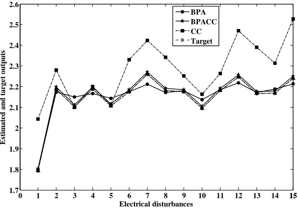
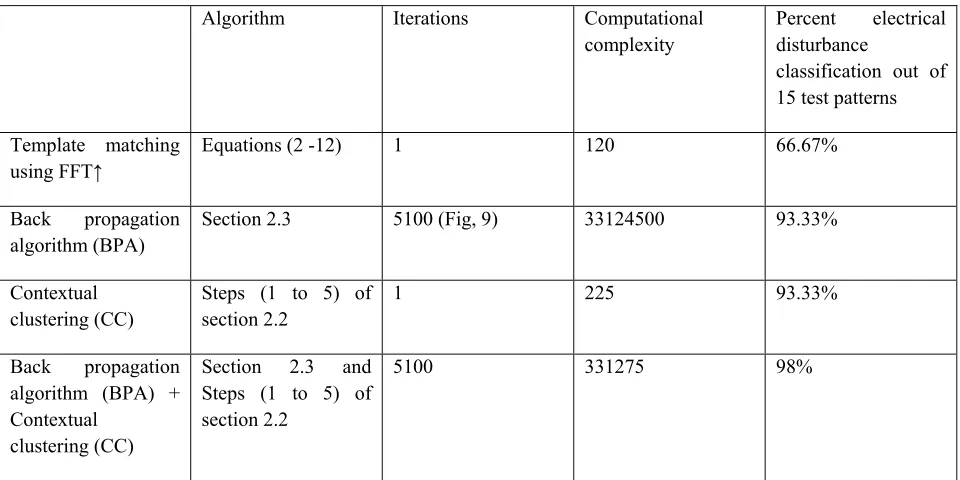
Figure 11 presents the performance comparison of the Back propagation algorithm and contextual output with the target values. The outputs of BPA is closer to the target values. The outputs of contextual clustering is deviating and not closer to target output. The combination of contextual clustering and BPA gives closer approximation to the target values. Table 6 presents performance comparison of results for the proposed algorithm. In this it can be notice the performance of BPACC is higher than that obtained from CC and BPA. This increased in results is specific for the data used in this work. The algorithm has to be verified for different ranges of electrical disturbances.

6.Conclusion

Table 6 Performance comparisons

Algorithm Iterations Computational

complexity

Percent electrical disturbance

classification out of 15 test patterns Template matching

using FFT↑

Equations (2 -12) 1 120 66.67%

Back propagation algorithm (BPA)

Section 2.3 5100 (Fig, 9) 33124500 93.33%

Contextual clustering (CC)

Steps (1 to 5) of section 2.2

1 225 93.33%

Back propagation algorithm (BPA) + Contextual

clustering (CC)

Section 2.3 and Steps (1 to 5) of section 2.2

5100 331275 98%

↑Computation involved in FFT is not considered for comparison of algorithm as the features extracted through FFT is used for all algorithms

References

[1] Aiello, M.; Cataliotti, A.; and Nuccio, S. (2005) ‘A Chirp-Z transform-based synchronizer for power system measurements’, IEEE Trans. Instrum. Meas, Vol.54, pp.1025–1032.

[2] Bhim Singh. et al, (1999) ‘A Review of Active Filters for Power Quality Improvement’, IEEE Trans On Industrial Electronics, Vol.46, pp.960-971.

[3] Brown. et al. (1996) ‘Distribution system reliability assessment using hierarchical Markov modeling’, IEEE Trans on Power Delivery,

Vol.2, pp.1929-1934.

[4] Dash, et al (1998) ‘A new approach to monitoring electric power quality’, Electric Power Systems Research, Vol.46, pp.11–20.

[5] Dash, P.K.; Jena, R.K.; and Salama, M.M.A. (1999) ‘Power quality monitoring using an integrated Fourier linear combiner and fuzzy expert system’, Electrical Power and Energy Systems, Vol. 21,pp.497–506.

[6] Eero Salli, et al (2001) ‘Contextual Clustering for Analysis of Functional MRI Data’, IEEE Trans On Medical Imaging, Vol.20,

pp.403-414.

[7] Elmitwally, A.; Abdelkader, S.; and El-Kateb, M. (2000) ‘Neural network controlled three-phase four-wire shunt active power filter’, IEE Proceedings of Generation, Transmission and Distribution, Vol.147, pp.87-92.

[8] Fonseca da Silva, et al (2004) ‘A new four parameter sine fitting technique, Measurement, Vol.35, pp.131–137.

[9] Leonowicz, Z.; Lobos, T;.and Rezmer, J. (2003) ‘Spectrum estimation of nonstationary signals in power systems’, International Conference on Power System Transients IPST, pp.1-6, New Orleans, USA.

[10] Mário Oleskovicz. et al (2009) ‘Power quality analysis applying a hybrid methodology with wavelet transforms and neural networks’,

Electrical Power and Energy Systems, Vol.31, pp.206–212.

[11] Murat Uyar.; Selcuk Yildirim.; and Muhsin Tunay Gencoglu. (2008) ‘An effective wavelet-based feature extraction method for classification of power quality disturbance signals’, Electric Power Systems Research, Vol.78, pp.1747–1755.

[12] Pradhan, A.K.; Routray, A.; and Sethi, D. (2004) ‘ Voltage phasor estimation using complex linear Kalman filter’, Eighth IEE International Conference on Developments in System Protection, Vol.1, pp. 24–27.

[13] Soliman, S.A.; and El-Hawary, M.E. (2000) ‘Measurement of power systems voltage and flicker levels for power quality analysis: a static LAV state estimation based algorithm’, Electrical Power and Energy Systems, Vol.22, pp.447–450.

[14] Solimana, S.A.; Mantawayb, A.H.; and El-Hawary, M.E. (2004) ‘Simulated annealing optimization algorithm for power systems quality analysis’, Electrical Power and Energy Systems, Vol.26, pp.31–36.

[15] Suja, S. and Jovitha Jerome. (2010) ‘Pattern recognition of power signal disturbances using S Transform and TT Transform’, International Journal of Electrical Power and Energy Systems, Vol. 32, pp.37-53.

[16] Suriya Kaewarsa.; Kitti Attakitmongcol.; and Thanatchai Kulworawanichpong. (2008) ‘Recognition of power quality events by using multiwavelet-based neural networks’, Electrical Power and Energy Systems, Vol.30, pp.254–260.

[17] Zheng, G, et al (2002) ‘Power quality disturbance classification based on rule-based and wavelet-multi-resolution decomposition’,

Elango M.K. has received his B.E degree in Electrical and Electronics

Engineering in 1997 from Madras University, Chennai and M.E.degree in Power System in 2004 from Faculty of Engineering and Technology, Annamalai University Chidhambaram. From 1997 till date he is working with K.S. Rangasamy College of Technology, Tiruchengode and pursuing his Ph.D degree at Anna University Chennai, India. His research interests are Application of Computational intelligent techniques, Power quality monitoring and Signal processing

Dr.Nirmalkumar.A, has received the B.Sc.(Engg.) degree from NSS College of