Page 196 www.ijiras.com | Email: [email protected]
Simulation Scenario For Digital Conversion And Line Encoding Of
Data Transmission
Olutayo Ojuawo
Department of Computer Science,
The Federal Polytechnic, Ilaro, Ogun State, Nigeria
Luis Binotto
M.Sc in Network and Information Security, Kingston University, London, United Kingdom
I. INTRODUCTION
The process described in this paper is one of the many possible scenarios in which an analog signal could be processed and transmitted. The aim is to illustrate, analyze and evaluate how an analog signal is treated, digitalized and then codified into one of the Line Coding schemes of the industry, 2B1Q, which is used in DSL (Digital Subscriber Line) to provide high-speed connection to the internet by using the telephone subscriber lines.
In this scenario, the original analog signal such as one created from a microphone or received using AM of FM modulation, prior to being digitalized, is analyzed in order to remove the noise product of any interference. A fast Fourier transform (FFT) calculates a sequence discrete Fourier transform (DFT) or it’s inverse. Fourier analysis converts a signal from its original domain (often time or space) to a representation in the frequency domain and vice versa. The FFT is used in this case in order to determine the frequencies of the compound signal and be able to design the appropriate transfer function which meets the specifications for the cut-off frequency of the filters observed in the FFT diagram. Once the filters are applied, a digitalization technique called Pulse Code Modulation (PCM) is used. A pulse modulation (PCM) technique is a technique in which the amplitude of an analog
signal is converted to a binary value represented as a series of pulses. Three basic processes integrate this stage: sampling, quantization, and encoding. The stream of bits obtained is the digital representation of the original analog wave. In order to be transmitted, that sequence of bits, or digital data, needs to be converted into digital signal by encoding it into the 2B1Q scheme (Two Binary, Two Quaternary).
II. FAST FOURIER TRANSFORM AND FILTERS Every possible waveform and function in existence can be generated by adding together different sets of sine waves. When an infinite number of sine waves of infinite small amplitudes are added together, it is possible to measure the density of frequencies. This density will be higher around some frequencies than others, and this is referred as frequency spectrum of a waveform. The DFT (Discrete Fourier transform), takes a discrete signal in the time domain x[t] and transform it into a discrete signal in the frequency domain (frequency spectrum). The transformation is given by the equation:
Abstract: Data communications encompass the transmission of data within media. Conversion from analog to digital involves series of processes in which noise serves as a disturbance in digital modulation. This paper describes a simulation scenario in which an analog signal is received, analyzed using Fast Fourier Transform (FFT), filtered to eliminate the noise and digitalized using PCM technique to be transmitted over the telephone lines. FFT is used to analyze the wave and design the filters to clear the wave before conversion from analog to digital. The simulation was implemented with Matlab codes.
Page 197 www.ijiras.com | Email: [email protected] Inverse transform:
N = Number of samples n = current sample considering xn = value of the signal at the time n
k = current frequency considering [0, N-1] Hz
Xk = amount of frequency k in the signal (Amplitude and
Phase. Complex number). (Isam, 2014)
The FFT (Fast Fourier Transform) is a faster version of the DFT. It is the speed and the discrete nature of the FFT that makes it possible to analyses a signal spectrum in real time and therefore the importance and the vast range of applicability of this algorithm. Figure 1 shows a compound signal and its corresponding frequency spectrum:
Figure 1: Compound signal and Frequency spectrum
The complex waveform (solid line) is composed of three waveforms (dotted lines) and those frequencies could be observed in the spectrum given by the FFT. The FFT is also useful to design digital filters. There is a correlation between time domain and frequency domain in the principles behind digital filters. For a signal in the time domain, a convolution operation can be done by performing a series of point by point multiplications. The convolution operation in the frequency domain is equivalent to multiply all frequency components in the passband by 1 and all frequency in the stop band by 0, as can be seen in the figure 2. (element14community, 2011)
Figure 2: FFT graph
There are two types of digital filters: Finite Impulse Response (FIR) and Infinite Impulse Response (IIR). Figure 3 shows the block diagram of each one:
FIR filters use only current and past input digital samples to obtain a current output value. No feedback is used. The general equation is given by (Van Veen, 2012) :
IIR filters uses current input samples values, as well as past inputs and outputs samples values to obtain current output. The general equation is given by (Van Veen, 2012) :
Z-1
a1
Z-1
a0
a2
yn
Xn
Xn-1
Xn-2
b1
b2
Z-1
Z-1 Z-1
a1
Z-1
a0
a2
yn
Xn
Xn-1
Xn-2
FIR Filter
IIR Filter
Figure 3: FIR and IIR Filters
Yn-1
Page 198 www.ijiras.com | Email: [email protected] The transfer function H(z) of FIR filters has only zeros
while IIR has zeros and poles and require less memory than FIR. In FIR filters linear phase is always possible, are stables due to they do not use feedback and the order can be high. In contrast, in IIR filters, the phase is difficult to control, can be unstable since feedback is used, consumes more power due to the use of more coefficients in the design but are more efficient. FIR filters are used as anti-aliasing, low pass, and baseband filters. IIR filters are used as band stop, bandpass functions. For both filters, the number of arithmetic operations needed per unit time is directly related to filter order (DT Filter Design: IIR Filters, 2006).
III. ANALOG TO DIGITAL CONVERSION AND LINE CODING SCHEME
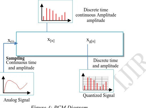
The most common technique to digitalize an analog signal is called Pulse Code Modulation (PCM). PCM has three processes as shown in figure 4:
Sampling
In 1949, Shannon published a paper called: “Communication in the presence of noise”, that masterpiece has had a huge impact on modern electrical engineering because describing how to convert an analog signal into a sequence of numbers which can be processed digitally.
Shannon Theorem: If a function f(x) contains no frequencies higher than (in radians per second), it is completely determined by giving its ordinates at a series of points spaced seconds apart. The reconstruction formula that complements the sampling theorem is:
A minimum sampling rate is therefore
samples/seconds; equivalently, for a given sampling rate fs, perfect reconstruction is possible at a series of point spaced a band limit . When a band limit is too high, the reconstructed signal exhibits imperfections and that is known as aliasing. The two thresholds, and fs/2, are respectively called the Nyquist rate and Nyquist Frequency. (Unser, 2000)
IV. QUANTIZING AND ENCODING
The result of sampling is a series of pulses (discrete time) with infinite amplitude values between the maximum and the minimum of the signal (continuous values) (Forouzan, 2013). Hence, quantization begins with the availability of analog samples in the range of . The quantization process replaces the magnitude of these samples with a value which is an approximation to the original amplitude in a set of discrete real numbers. (Gerso, 1977). More generally, we can define a quantizer as consisting of a set of intervals or cells , where the index set I is ordinarily a collection of consecutive integers beginning with 0 or 1, together with a set of reproduction values or points or levels , so that the overall quantizer is defined by for , this can be written as:
where 1S(x) is 1 if and 0 otherwise (Gray, 1998).
It is possible to establish a classification of the quantizer as Fixed-Rate Scalar Quantization, Scalar Quantization with Memory, Variable-Rate Quantization, and Vector Quantization. Fixed-Rate Scalar Quantization has their origins in pulse-code modulation (PCM) that was the first digital technique for conveying an analog signal (principally telephone speech) over an analog channel (typically, a wire or the atmosphere) (Gray, 1998).
The following are the steps for Fixed Scalar Modulation: Let’s, Vmax and Vmin, the normalized values of magnitudes
maximum and minimum, n, the number of resolution bits and L, the number of levels.
Divide the range from Vmax to Vmin into L zones to
calculate the delta between each zone:
For each Vi
The quantized value (Vq) of the Vi
The process induces an error that depends on the number of levels. The input values to the quantizer are the real values, the output values are the approximated values, and this difference is called quantization error. The contribution of the quantization error to the SNRdB of the signal depends on of the
number of levels and is given by the formula (Forouzan, 2013):
Figure 5 shows an example with 8 samples/period, n=2 resolution bits, L=4 and .
Figure 4: Quantization and encoding Figure 4: PCM Diagram
Sampling Quantizing Encodin g x(t)
Discrete time and amplitude
Analog Signal Continuous time
and amplitude
PAM Signal
x[n] xg[n]
Discrete time continuous Amplitude
amplitude
Page 199 www.ijiras.com | Email: [email protected] Magnitudes 0 0.7 1 0.7 0
-0.7
-1 -0.7
Index (I) 2 3 3 3 2 0 0 0
1 1.5 1.5 1.5 1 0 0 0
Vq 0 0.5 0.5 0.5 0 -1 -1 -1
Error 0
-0.2 -0.5
-0.2
0 0.3 0 0.3 Binary Code 10 11 11 11 10 00 00 00
Table 1
V. LINE CODING
This s the process of converting digital data to a digital signal, which means to convert a stream of bits to a digital signal and be able to transmit it over a wire. There are five categories of coding schemes such as Unipolar (e.g.: NRZ), Polar (e.g.: NRZ, RZ, Manchester, diff Manchester), Bipolar (e.g.: AMI), Multilevel (e.g.: 2B1Q, 8B6T, 4D-PAM5), Multi-transition (e.g.: MLT-3).
The scheme 2B1Q (2 binary 1 Quaternary), uses a sequence of 2 bits to encode one signal element belonging to a four-level signal (Forouzan, 2013). The patterns and its respective voltage conversion are as follow:
00: -3, 01: -1, 10: +3, 11: +1
Figure 5 shows the 2B1Q encoding scheme for the stream of bits of figure 4.
Figure 5: 2B1Q scheme encoding
VI. IMPLEMENTATION AND ANALYSIS
For the scenario, three sinusoidal waves were adding together and Gaussian noise was added to the resulting signal.
S1 = sin(2*pi*f*t); S2 = 1/3*sin(2*pi*3*f*t); S3 = sin(2*pi*26*f*t); S4 = S1+S2+S3;
SR = awgn(S4,5,'measured');
SR, represent a signal that could have been generated by a microphone or received from an analog source. The SR plot is shown in figure 6.
Figure 6: Signal for analysis
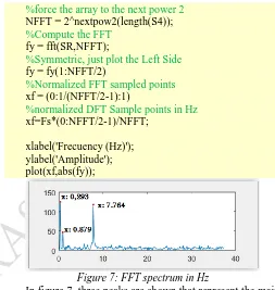
The goal is to apply the FFT in order to determine the spectrum and design the respective filter to eliminate the undesired frequencies, in this case, the noise. The FFT function, perform better if the samples of the signal are multiples of 2. This can be achieved using 2^nextpow2(). One important factor to consider in the fft, is the symmetry, it comes about due to the use of a complex exponential in the DFT, so it is necessary to plot the values until N/2, where N is the number of samples in the FFT. The code to compute the FFT in Matlab is:
%force the array to the next power 2 NFFT = 2^nextpow2(length(S4)); %Compute the FFT
fy = fft(SR,NFFT);
%Symmetric, just plot the Left Side fy = fy(1:NFFT/2)
%Normalized FFT sampled points xf = (0:1/(NFFT/2-1):1)
%normalized DFT Sample points in Hz xf=Fs*(0:NFFT/2-1)/NFFT;
xlabel('Frecuency (Hz)'); ylabel('Amplitude'); plot(xf,abs(fy));
Figure 7: FFT spectrum in Hz
In figure 7, three peaks are shown that represent the main frequencies of the SR, the rest, represent frequencies induced by noise. The next step is to implement filters and remove the undesired frequencies. Two filters were implemented for this case are low pass filters and the stop band filters. To make the code more independent when the original signal is changed, an adaptive filter function was coding (definefilters.m). This function groups the harmonics (helping by a given threshold) and decides the types of filters that should be used (low pass or stop band), returning the values of the bands that have to be implemented for the filters. To find the peaks (that represent the harmonics of the composed wave) the Matlab function findpeaks() was used. It uses the array of values and two parameters: MinPeakHeight and minPeak. The former tells the function to consider a Peak depends on its height. The latter is a variable, in which is specified the minimum height for what is considered a peak. These array of Peak locations are passed to the function definefilters() to the group and calculate the bands and the type of filters needed to be applied. The code in Matlab is:
%locate the numbers of Peaks of the FFT minPeak = (max(fy) - mean(fy))/2;
[peaks, PeakLoc]=
findpeaks(fy,'MinPeakHeight',minPeak);
% Agrupate peaks in groups and calculate the bands for auntomatic
% configuration
Page 200 www.ijiras.com | Email: [email protected] The filters implemented were Butterworth type filters and
the function used in Matlab was butter() It receive the order, the cut-off frequency and the type of filter (calculated previously by the function definefilters()), and return the a and
b coefficients.
To show the frequency response of the system it is necessary to plot H(z), that is calculated with the function
freqz(). The code in Matlab to implement filters is:
%Design a low pass filter using butterworth design technique
lowband1 = xf1(low)+0.03; [B A]= butter(20, lowband1, 'low'); H = freqz(B,A,floor(NFFT/2));
% Design a band reject filter using buterwork design technique
if (length(stop) > 1)
stopband1 = xf1(stop(1))+0.05; stopband2 = xf1(stop(2))-0.04;
[b_stop a_stop] = butter(8, [stopband1 stopband2], 'stop');
H_StopBand = freqz(b_stop,a_stop,floor(NFFT/2)); end
Figure 8 shows the FFT along with the filters designed.
Figure 8: FFT spectrum Vs Filters
The signal filtered is shown in figure 9:
Figure 9: Filtered signal
Continuing with the scenario, once the signal is filtered it can be digitalized in order to be transmitted.
The signal must be sampling at least 2*fmax (Nyquist rate).
To find fmax is necessary to find the peak with the highest
frequency from the values returned (PeakLoc) by the function
findPeaks(). The position of the highest frequency will correspond with the same position in xf that represent the maximum frequency of the signal.
fmax = PeakLoc(length(PeakLoc)); fmax = xf(fmax);
The sampling frequency, in this case, will be N (number of samples/period) * fmax
To quantize the signal, the steps for Fixed Scalar Modulation described above are applied. The code in Matlab is shown as follow:
% Quantize a signal to "b" bits. % Index
xq=floor((x+1)*2^(b-1)); % Index*Delta
xq=xq/(2^(b-1)); % Value in x quantize
xq=min(x)+xq;
Figure 10 shows the samples and quantized values for the signal SR:
Figure 10: Sampling and Quantization
The last process of PCM is encoding in which each sample is matched with a specific level and changed into a world of b bits. The code in Matlab to implement this step is:
% Decimal to Binary Conversion levels=floor((x+1)*2^(b-1));
L = length(levels); % Data Elements of b bits for(i=1:L)
j = ((i-1)*b)+1;
BinData(j:j+b-1) = dec2binary(levels(i),b); end
Once the analog to digital conversion is done, in order to transmit the data over the wire, it is necessary to use the appropriate scheme depending on the type of medium that will be use. In this case the scheme use was 2B1Q. The code in Matlab that simulate the output is described as follows:
%Using the 2B1Q encoding scheme j =1;
for(i = 1:2:length(BinData))
x = BinData(i)*10 + BinData(i+1); switch x
case 00
scheme_2b1q(j) = -3; case 01
scheme_2b1q(j) = -1; case 10
scheme_2b1q(j) = 3; case 11
scheme_2b1q(j) = 1; end
j=j+1; end
%Plot the coding scheme 2B1Q L = length(scheme_2b1q);
[cod_xdata, cod_ydata] =
stairs([scheme_2b1q,scheme_2b1q(end)]); sub23 = subplot(4,1,3);
plot(sub23,cod_xdata,cod_ydata)
VII.CONCLUSION
Page 201 www.ijiras.com | Email: [email protected] broad range of applications in the communication area, the
concepts explained in this paper are just the base to understand the applications for the analysis in the frequency domain. Similarly, the process to digitalize a signal using PCM is the first step to digging deeper into this area that involves sampling, quantization, and encoding. Theoretically, the sampling theorem of Shannon states that the rate samples must satisfy the criterion fc≥2fm, but with the purpose of increase the
accuracy in the reproduction of the original signal the sampling frequency is usually higher, sacrificing bandwidth at expense of accuracy.
Once the signal is sampled, quantized and encoded in a stream of bits, in order to be transmitted, it needs to be transforming from digital data to a digital signal. The parameters of voltages used, and the representation of bits is defined by the coding scheme. In this case, the scheme 2B1Q was used to simulate the transmission through the telephone lines (DSL).
REFERENCES
[1] DT Filter Design: IIR Filters. (2006). 1st ed. [ebook] Massachusetts Institute of Technology. Available at: [2]
http://ocw.mit.edu/courses/electrical-engineering-and-computer-science/6-341-discrete-time-signal- processing-fall-2005/lecture-notes/lec08.pdf [Accessed 02 Sept. 2016].
[3] Element14community, (2011). Digital Filters Part 1. [video] Available at:
https://www.youtube.com/watch?v=loHy8v9A8LY [Accessed 30 Sept. 2016].
[4] Forouzan, B. and Fegan, S. (2007). Data communications and networking. New York: McGraw-Hill Higher Education.
[5] Gerso, A. (1977). Quantization. [online] Available at: http://ieeexplore.ieee.org.ezproxy.kingston.ac.uk/stamp/st amp.jsp?tp=&arnumber=1089500.
[6] Gray, R. (1998). Quantization. IEEE TRANSACTIONS ON INFORMATION THEORY, [online] 44. Available at: http://ieeexplore.ieee.org.ezproxy.kingston.ac.uk/stamp/st amp.jsp?tp=&arnumber=720541.
[7] Isam, A. (2014). Understanding Fourier Series, Theory + Derivation. [video] Available at: https://www.youtube.com/watch?v=le_gMPJFyJ8&ebc= ANyPxKrYIZm9sgq5cf8ApYVHuu2gV5jPZ5TvjodFgAc
4nfWuisqpPErsM9yR-CytRAanOOV5-S1ufDimUe61jaUHvZh0XkNSg [Accessed 30 Aug. 2016].
[8] Unser, M. (2000). Sampling-50 years after Shannon.
Proceedings of the IEEE, 88(4), pp.569-587.
[9] Van Veen, B. (2012). Overview of FIR and IIR Filters. [video] Available at: