An Efficient Concept-based Mining Model for
Deriving User Profiles
P. Sasikala
V. Vidhya
PG Research Scholar
Faculty of Computer Science and Engineering
Sri Venkateswara College of Sri Venkateswara College of
Engineering Engineering
ABSTRACT
User profiling forms the basis for search engine personalization applications. Search engines are personalized so that they optimize the retrieval quality of user queries. User profiling done through concept-based mining identifies terms that render conceptual meaning as well as unimportant terms. Both positive and negative preferences from such conceptual terms are used in creating the user profiles and such profiles built based on both the preferences of a user reflect his/her interests at finer details.
Based on these accurate and up-to-date user profiles, relationships between users can be mined to perform Collaborative Filtering (CF) thereby allowing users with the same interests to share their profiles. Collaborative filtering filters information about a user based on a collection of user profiles that are already built from the extracted preferences. Users having similar profiles may share similar interests. The concept-based search enhanced by Collaborative Filtering improves the relevancy of search results by making automatic predictions about the interests of a user by collecting similar user profiles.
General Terms
Information retrieval, Search engine personalization, Web mining
Keywords
Clustering, Collaborative Filtering, Personalization, Query formulation, User profiles, Personality diagnosis
1.
INTRODUCTION
Today’s web search engines are still following the paradigm of keyword-based search. This is the best choice for large scale search engines in terms of throughput and scalability but it inherently limits the ability to accomplish more meaningful query tasks. It captures only user’s document preferences but the most relevant documents to a query may not have the query keyword at all and hence the user may not be able to retrieve these documents even when they were much more relevant to the searched query.
Also most commercial search engines return roughly the same results repeatedly for the same query without considering the user’s real interest. Most of the queries submitted to search engines tend to be short and ambiguous and hence they are not likely to be able to express the user’s precise needs. For example, a person may use the query “apple” to find information about the fruit apple, while it also refers to apple computer. So depending on the user’s search interest, the most relevant document pertaining to his search must be retrieved. This is the key feature of search engine personalization.
Search Engine Personalization aims to improve the retrieval quality of search engines. The key success factors of a search are Reliability, Ease/Speed of use.
A good user profiling strategy is an essential and fundamental component in search engine personalization and thus helps in improving the relevancy of search results.
Most personalization methods focused on the creation of a single profile for a user and applied the same profile to all of the user’s queries. Different queries from a user should be handled differently because a user’s preferences may vary across queries. Personalization strategies such as [1], [2], [7], [9], [12], [13], [14] employed a single user profile for each user in the personalization process.
Existing click through based user profiling strategies can be categorized into document-based and concept-based approaches. They both assume that user clicks can be used to learn about users’ interests. Document-based profiling methods try to estimate users’ document preferences (i.e., users are interested in some documents more than others)[1], [2], [7], [9], [13].
On the other hand, concept-based profiling methods aim to derive topics or concepts that users are highly interested in [12], [14]. Concept-based search captures user’s conceptual needs and provides the user with more relevant documents to the searched query.
Most existing user profiling strategies only consider documents that users are interested in (i.e., users’ positive preferences) but ignore documents that users dislike (i.e., users’ negative preferences). In reality, positive preferences are not enough to capture the fine grain interests of a user. There are document-based methods that consider both users’ positive and negative preferences but there are very few concept-based methods that considered both positive and negative preferences in deriving user’s topical interests[18]. Personalization strategies such as [9], [13], [15] include negative preferences in the personalization process, but they all are document-based, and thus, cannot reflect users’ general topical interests. Profiles built on both positive and negative user preferences can represent user interests at finer details. Profiles with negative preferences can increase the separation between similar and dissimilar queries.
This paper improves the relevancy of search results by combining concept-based user profiling strategies with collaborative filtering.
about which DVD a user should like given a partial list of that user's tastes.
Memory-based collaborative filtering mechanism uses user preferences to compute similarity between several users. Typical examples of this mechanism are neighborhood based CF and item-based or user-based top-N recommendations. The advantages with this approach include: It is easy to create and use, new data can be added easily and incrementally. Several disadvantages with this approach: It depends on human preferences and its performance decreases when data gets sparse. This prevents the scalability of this approach and has problems with large datasets. It iterates through all the known users making the whole process complex.
Model–based collaborative filtering uses the existing users as models for the active user but thus iterates through all the known users. Hence to reduce complexity, iterations are done over only a selected portion of the existing users. Models are Bayesian Networks, clustering models, latent semantic models such as singular value decomposition, probabilistic latent semantic analysis, Multiple Multiplicative Factor, Latent Dirichlet allocation and markov decision process based models.
Several advantages of this approach are:
1) It works for sparse data. This improves scalability with large data sets.
2) It improves the prediction performance and are used to make predictions for real data.
The disadvantage with this approach is the cost involved in building the model.
Hybrid collaborative filtering combines the memory-based and the model-based CF algorithms. The limitations of native CF approaches are counteracted in hybrid CF. It improves the prediction performance and overcomes the CF problems such as sparsity and loss of information.
2.
USER PROFILING
Evaluating user preferences from web search results obtained by issuing a query to the search engine is crucial for search engine development, deployment and maintenance. The browsing behaviors of web search users are analysed to predict user preferences. Accurate modeling and interpretation of user behavior helps in ranking, web search personalization and other tasks.
User profiling strategies can be broadly classified into two approaches: document-based profiles and concept-based profiles.
2.1
Document Based Methods
Document based profiling methods try to identify users’ document preferences i.e., those documents that the users are more interested in than others. They do not reflect user’s topical interests.
2.1.1
Joachims Method
Joachims’ method assumes that when a user is provided with a set of search results for his current query, the user would scan the search results from top to bottom. If a user has skipped a document 𝑑𝑖 at rank i before clicking on document 𝑑𝑗 at rank j, it implies that the user must have scanned the
document 𝑑𝑖 and because the document does not reflect his interests, he has decided to skip it. Thus the user has preferred document 𝑑𝑗 more than the document 𝑑𝑖 (i.e.) 𝑑𝑗 < 𝑟′𝑑𝑖 in
ranking where 𝑟′ is the user’s preference order of the documents from the set of retrieved search results [18].
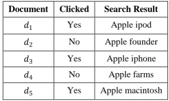
By deploying Joachims’ method on a set of sample click through data, document preference pairs can be obtained. Table 1. Click through data
Table 1 shows an example of click through data where out of 5 documents, 3 documents have been clicked by user and might reflect his preferences.
Table 2. Obtaining document preference pairs
Table 2 shows how document preference pairs are obtained using Joachims method. It is inferred that the document 𝑑3 is preferred than 𝑑2 and document 𝑑5 is preferred than documents 𝑑2 and 𝑑4.
Joachim’s user profile consists of a set of weighted features. After the document preference pairs are obtained, a Ranking Support Vector Machine (RSVM ) is employed to learn the user behavior model as a set of weighted features
2.1.2
Spying With Novel Voting Procedure
Ng et al.[13] proposed an algorithm which combines a spying technique together with a novel voting procedure to determine users’ document preferences from the Click through data. It also employed the RSVM algorithm to learn the user behavior model as a set of weighted features.
2.1.3
Cleaned Up Click through Data
Agichtein et al.[1] suggested that explicit feedback (i.e., individual user behavior, click through data, etc.) from search engine users is noisy. It may be due to the bias of user click distribution towards top ranked results.(i.e) those search results that are higher in the ranking may have been assumed to be more relevant and user would have clicked that document without knowing if it is really relevant to his search. To resolve the bias, Agichtein suggested that the click through data be cleaned up with the aggregated “background” distribution .A scalable implementation of neural networks is then employed to learn the user behavior model from the cleaned click through data.
2.2
Concept Based Methods
Concept-based methods automatically derive users’ topical interests by exploring the contents of the users’ browsed documents and search histories.
Document preference pairs for 𝑑1
Document preference pairs for 𝑑3
Document preference pairs for 𝑑5
Empty set 𝑑3 < 𝑟′𝑑2 𝑑5 < 𝑟′𝑑2
𝑑5 < 𝑟′𝑑4
Document Clicked Search Result
𝑑1 Yes Apple ipod
𝑑2 No Apple founder
𝑑3 Yes Apple iphone
𝑑4 No Apple farms
2.2.1
ODP Based Profiling
Liu et al [12] proposed a user profiling method based on users’ search history and the Open Directory Project (ODP). The user profile is represented as a set of categories and for each category, there are a set of keywords with weights. The categories stored in the user profiles serve as a context to disambiguate user queries. If a profile shows that a user is interested in certain categories, the search can be narrowed down by providing suggested results according to the user’s preferred categories.
2.2.2
Profiling Based On Magellan’s Concept
Hierarchy
Gauch and Speretta [8] proposed a method to create user profiles from user-browsed documents. User profiles are created using concepts from the top four levels of the concept hierarchy created by Magellan. A classifier is employed to classify user browsed documents into concepts in the reference ontology.
2.2.3
Hierarchical User Profiles
Xu et al.[17] proposed a scalable method which automatically builds user profiles based on users’ personal documents (e.g., browsing histories and e-mails). The user profiles summarize the users’ interests into hierarchical structures. The method assumes that the terms that exist frequently in user’s browsed documents represent topics that the user is interested in. Frequent terms are extracted from users’ browsed documents to build hierarchical user profiles representing users’ topical interests. It automatically extracts possible topics from users’ browsed documents and organizes the topics into hierarchical structures.
Liu et al.[12] and Gauch and Speretta [8] both use reference ontology (e.g., ODP) to develop the hierarchical user profiles. The major advantage of dynamically building a topic hierarchy is that new topics can be easily recognized and extracted from documents and added to the topic hierarchy whereas reference ontology such as ODP is not always up-to-date.
3.
OVERVIEW OF THE PAPER
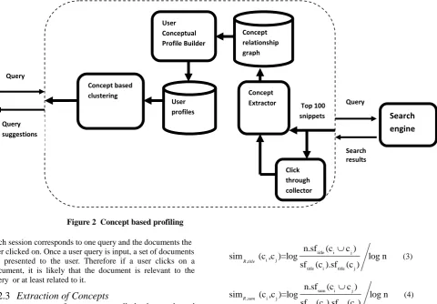
This paper deals with combining concept-based user profiling strategies with collaborative filtering. The first step is Concept Extraction in the user profiling process. The web snippets are retrieved from the search results returned by the search engine and concepts are extracted. The related concepts are identified and the concept relationship graph is drawn. After the concept preference pairs are identified, a ranking SVM algorithm is employed to learn the user’s preferences, which is represented as a weighted concept vector. Frequent terms are extracted from users’ browsed documents to build user profiles representing users’ topical interests.
A personalized concept-based clustering algorithm employs a query-concept bipartite graph G and is used to classify ambiguous queries into different query clusters. Concept-based user profiles are employed in the clustering process to achieve personalization effect. Concepts with interestingness weights greater than zero in the user profile are linked to the query with the corresponding interestingness weight in G. Now accurate user profiles are created with each user’s queries and their preferred concepts. Figure 2 shows the overall system architecture for creating concept-based user profiles.
Collaborative filtering (CF) is then applied that filters information for a user based on a collection of user profiles. It
computes similarity between user profiles and predicts preferences for the current user based on other similar users’ profiles.
4.
CONCEPT EXTRACTION
Concept Extraction is the first step in the user profiling process. The web snippets are retrieved from the search results returned by the search engine and concepts are extracted. The related concepts are identified and the concept relationship graph is drawn.
4.1
Basic Working Of Search Engines
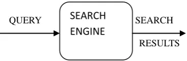
The user opens the home page of a search engine and enters a query. The web search engine searches for the user’s query and display the results page.
QUERY SEARCH
RESULTS
Figure 1 Basic working of search engines
Figure 1 shows the basic working of search engines. The title, summary and URL of a web page form the snippets. These snippets have to be retrieved from the search results which are got by giving a query to the search engine.
4.2
Concept Extraction From Web
Snippets
4.2.1
General Methodology
The most frequently occurring words in snippets are considered to be the important keywords of the retrieved snippets. To compute the interestingness of a particular keyword extracted, Support formula is used.
𝑠𝑢𝑝𝑝𝑜𝑟𝑡 𝑐𝑖 = 𝑠𝑓 𝑐𝑖 /𝑛 ∙
c
i (1)where n is the total number of web-snippets returned,
𝑠𝑓 𝑐𝑖 is the snippet frequency of the keyword or phrase 𝑐𝑖
(i.e., the number of web-snippets containing 𝑐𝑖 ) and 𝑐𝑖 is the number of terms in the keyword or phrase 𝑐𝑖. It resembles the problem of finding frequent item sets in data mining. When a user submits a query to the search engine, a set of
web snippets are returned to the user for identifying the relevant items. The assumption is that if a keyword or a phrase appears frequently in the web snippets of a particular query, it represents an important concept related to the query because it occurs together with the query in the top documents. Support formula given by equation (1) measures the interestingness of a particular keyword or phrase with respect to the returned web snippets arising from a query q.
4.2.2
Preprocessing
The data to be preprocessed is from a large set of user logs and also from topmost web search results. From the user logs, a query session is defined as follows:
Session : D<query text> [clicked document]
Figure 2 Concept based profiling
Each session corresponds to one query and the documents the user clicked on. Once a user query is input, a set of documents are presented to the user. Therefore if a user clicks on a document, it is likely that the document is relevant to the query or at least related to it.
4.2.3
Extraction of Concepts
To extract concepts for a query q, all the keywords and phrases are extracted from the web snippets returned by the query along with the concepts from clicked documents. After obtaining a set of keywords or phrases, compute the support for all. If the support of a keyword or a phrase 𝑡𝑖 is bigger
than a threshold(say 0.003), 𝑡𝑖 may be treated as a concept for the query q.
4.3
Identification Of Related Concepts
To find relationship between retrieved concepts, signal-to-noise ratio formula from data mining is applied .This establishes similarity between terms t1 and t2. The similarity
value always lies between [0, 1] and it can be used directly.
1 2 1 2
1 2
n.df(t t )
sim(t ,t )=log log n
df(t ).df(t )
(2)
Equation (2) gives similarity between two terms where n is the number of documents in the corpus, df(t1U t2) is the joint
document frequency of t1 and t2 and df(𝒕𝟏) is the document
frequency of the term 𝒕𝟏.
Two concepts 𝑪𝒊, 𝑪𝒋 could occur together in a web-snippet in the following situations: 1) 𝑪𝒊 and 𝑪𝒋 occur together in the title, 2) 𝑪𝒊 and 𝑪𝒋 occur together in the summary, or 3) 𝑪𝒊
occurs in the title, while 𝑪𝒋 occurs in the summary (or vice
versa ).Similarities for the three different cases are computed using the following Equations (3) , (4) and (5).
title i j
i j ,
title i title j
n.sf (c c )
sim (c ,c )=log log n
sf (c ).sf (c )
R title
(3)
sum i j
, i j
sum i sum j
n.sf (c c )
sim (c ,c )=log log n
sf (c ).sf (c )
R sum
(4)
other i j
, i j
other i other j
n.sf (c c )
sim (c ,c )=log log n
sf (c ).sf (c )
R other
(5)
where 𝑠𝑓𝑡𝑖𝑡𝑙𝑒(𝑐𝑖∪ 𝑐𝑗) and 𝑠𝑓𝑠𝑢𝑚 (𝑐𝑖∪ 𝑐𝑗) are the joint snippet frequencies of the concepts 𝑐𝑖 and 𝑐𝑗 in Web-snippets’ titles
and summaries, 𝑠𝑓𝑡𝑖𝑡𝑙𝑒 (c) and 𝑠𝑓𝑠𝑢𝑚(c) are the snippet
frequencies of the concept c in Web-snippets’ titles and summaries, 𝑠𝑓𝑜𝑡ℎ𝑒𝑟(𝑐𝑖∪ 𝑐𝑗) is the joint snippet frequency of
the concepts 𝑐𝑖 in a web-snippet’s title and 𝑐𝑗 in a Web-snippet’s summary (or vice versa), and 𝑠𝑓𝑜𝑡ℎ𝑒𝑟(c) is the snippet frequency of concept c in either Web-snippets’ titles or summaries.[18]
The following formula is used to obtain the combined similarity 𝑆𝑖𝑚𝑅(𝑐𝑖,𝑐𝑗) from the three cases, where α+β+γ=1 to ensure that 𝑆𝑖𝑚𝑅(𝑐𝑖,𝑐𝑗) lies between [0, 1].
.A concept graph is then built for the query. The nodes are the concepts extracted from the query and the links are created between concepts having 𝑠𝑖𝑚𝑅(𝐶𝑖, 𝐶𝑗) > 0.
Equation (6) gives the combined similarity scores.
j , i j , i j
, i j
i,
sim C C =α.sim C ,C +β.sim C ,C
+ γ.sim C ,C
R R title R sum
R other
(6)
Search engine
Query suggestions
Query
QUER
Y
Top 100 snippetsConcept Extractor
Click through collector Concept
relationship graph
Concept based clustering
User profiles User Conceptual Profile Builder
Query
QUE
RY
5.
CREATION OF USER CONCEPT
PREFERENCE PROFILES
To increase the relevance of search results, personalized search engines create user profiles to capture the users’ personal preferences and as such identify the actual goal of the input query.
5.1
Constructing a Hierarchical User
Profile
The user profiles are automatically built based on users’ personal documents (e.g., browsing histories and e-mails). The users’ interests are summarized into hierarchical structures by the user profiles. The method assumes that terms that exist frequently in user’s browsed documents represent topics that the user is interested in. Frequent terms are extracted from users’ browsed documents to build hierarchical user profiles representing users’ topical interests. From user’s browsed documents, it automatically extracts possible topics and the topics are organized into hierarchical structures. This focus on frequent terms limits the dimensionality of the document set and thus provides a clear description of users’ interest. In the hierarchy, general terms with higher frequency are placed at higher levels, and specific terms with lower frequency are placed at lower levels.
D represents the set of all personal documents and each document has a list of terms. D(t) denotes all documents covered by term t, (i.e.), all documents in which t appears, and |D(t)| represents the number of documents covered by t. A term t is frequent if |D(t)| ≥ minsup, where minsup represents the minimum number of documents in which a frequent term is required to occur. Each frequent term indicates a possible user interest.
For a term 𝑡𝐴, any document covered by 𝑡𝐴 is assumed to be a natural evidence of users’ interests on 𝑡𝐴. Also, documents
covered by term 𝑡𝐵 that either represents the same interest as 𝑡𝐴 or a child interest of 𝑡𝐴 can also be regarded as supporting documents of 𝑡𝐴 .Hence supporting documents on
term 𝑡𝐴,denoted as S(𝑡𝐴), are defined as the union of D(𝑡𝐴) andall D(𝑡𝐴), where either 𝑆𝑖𝑚(𝑡𝐴, 𝑡𝐵) > 𝛿 or P 𝑡𝐴|𝑡𝐵 > δ is satisfied.
The algorithm automatically builds a hierarchical profile in a top-down fashion. The profile is represented by a tree structure, where each node is labeled a term t, and associated with a set of supporting documents S(t). Starting from the root, nodes are recursively split until no frequent terms exist on any leave nodes. First documents are scanned once and all frequent terms are sorted in a descending order of (document) frequency. For each frequent term t, the initial supporting documents S(t) are set as D(t). All frequent terms are checked separately in a descending order of frequency. A node labeled term t is created. Supporting documents S(t) is attached with each node labeled t.
5.2
Click- Based Method
When a Web-snippet 𝑆𝑗 has been clicked by a user, the weight
𝑊𝐶𝑖 of concepts 𝐶𝑖 appearing in 𝑆𝑗 is incremented by 1. For
other concepts 𝐶𝑗 that are related to 𝐶𝑖 on the concept
relationship graph, they are incremented according to the similarity score .The related concepts have their weights increased based on the similarity score.
The following formulas capture a user’s degree of interest on the extracted concepts 𝐶𝑖, when a Web-snippet 𝑆𝑗 is clicked by the user .
Click( ) => C
s
j iS W = W + 1j , Ci Ci (7)j j
R
j => , C C sim i j
Click(S ) CiSj W = W + (C ,C )
R
if sim (C ,C ) i j > 0 (8) Equations (7) and (8) computes interestingness of the user on the extracted concepts where 𝑆𝑗 is a Web-snippet, 𝑊𝐶𝑖 represents the user’s degree of interest on the concept 𝐶𝑖
and 𝐶𝑗 is the neighborhood concept of 𝐶𝑖 .
For example , when the user searches for a query “apple”, the concepts derived from the concept extraction method contains “macintosh,” “ipod,” and “fruit.” If the user is indeed interested in “apple” as a fruit and clicks on pages containing the concept “fruit,” the user profile represented as a weighted concept vector should record the user interest on the concept “apple” and its neighborhood (i.e., concepts which having similar meaning as “fruit”), while unrelated concepts such as “macintosh,” “ipod,” and their neighborhood must be termed to be of low preference.
5.3
Spy NB-C Method
Spy NB assumes that unclicked pages could be either relevant or irrelevant to the user. Therefore, SpyNB treats clicked pages as positive samples and unclicked pages as unlabeled samples in the training process. The problem of finding user preferences also includes identifying from the unlabeled set reliable negative documents that are considered irrelevant to the user.
The “Spy” technique includes a novel voting procedure into a Naive Bayes classifier to derive reliable negative examples from the unlabeled set. Let “+” and “-” denote the positive and negative classes, and D = d1, d2... dn , a set of N
documents in the search result list.[16]
For each search result, Spy NB first extracts the words that appear in the title, abstract, and URL, creating a word vector (w1, w2... wM). Then, a Naive Bayes classifier is built by
estimating the prior probabilities (Pr(+)and Pr(-)) and likelihoods (Pr(wj|+)and Pr(wj|-).
The training data only contain positive and unlabeled examples (without negative examples). Thus, the “Spy” technique is employed to learn a Naive Bayes classifier. A set of positive examples S is selected from P andmoved into U as “spies” to train a classifier using the Naive Bayes algorithm . The resulting classifier is then used to assign probabilities Pr(+|d) to each example in U ᴜ S, and an unlabeled example in U is selected as a predicted negative example (PN) if its probability is less than Ts. In the search engine context, most
users would only click on a few documents (positive examples) that are relevant to them. Thus, only a limited number of positive examples can be used in the classification process, lowering the reliability of the predicted negative examples (PN).[16]
To resolve the problem, every positive example pi in P is used
as a spy to train a Naive Bayes classifier. Consequently, n predicted negative sets (PN1, PN2... PNn) are created with the
positive and predicted negative samples from the Spy NB, page preferences can be obtained.
Spy NB-C [18] generalizes page preferences into concept preferences. Specifically, concept preference pairs are obtained by assuming that concepts C(dj) in the positive
sample dj are more relevant than concept C(di) in the
predicted negative sample dj (i.e., C(dj)<r’ C(di)). Finally,
RSVM training is applied on the extracted concept preferences to learn a user profile PSpyNB-C which is
represented as a set of weight features.
The following steps show how spying is done to identify negative samples from unlabeled samples.
1)Set of positive samples are considered. 2)Set of unlabeled samples are considered. 3)Train the Naïve Bayes Classifier .
4)Identify the positive samples from unlabeled samples using the classifier and the rest of the unlabeled samples are considered to be negative.
The voting procedure retrieves reliable negative sets. It combines n predicted negative sets into a final negative sample.
5.4
Ranking SVM
After the concept preference pairs are identified, a ranking SVM algorithm [18] is employed to learn the user’s preferences, which is represented as a weighted concept vector.
Given a set of concept preference pairs T, ranking SVM aims at finding a linear ranking function f(q,c) to rank the extracted concepts so that as many concept preference pairs in T as possible are satisfied. f(q,c) is defined as the inner product of a weight vector w and a feature vector of query concept mapping ф(q,c), which describes how well a concept c matches the user’s interest for a query q.
The feature vector
ф(q,c) = [Feature_ c1, Feature_ c2 ,... ,Feature_ cn]
for the ranking SVM training is composed of all the extracted concepts for a query q.
For each concept ci, a feature vector is created
ф(q,ci)=[Feature_c1,Feature_c2,...,Feature_cn] (9)
The concept preference pairs together with the feature vectors serve as the input to the ranking SVM algorithm. The ranking SVM algorithm outputs a weight vector W. The weight vector
W=(WFeature-C1,WFeature-C2,...,WFeature-Cn) (10)
determines the user preferences on the extracted concepts. For all the concepts c1 , c2,... ,ci extracted for the query q, the user
preferences are stored in the corresponding weight values
WFeature-C1,WFeature-C2,... ,WFeature-Cn creating a concept
preferenceprofile .
6.
QUERY CLUSTERING
Query Clustering is the process to classify ambiguous queries in to different Query clusters.
6.1
General Query clustering algorithm
A query clustering algorithm mines a collection of user transactions with a search engine to discover clusters of similar queries and similar URLs. The information exploited is "clickthrough data": each record consists of a user's query
to a search engine along with the URL which the user selected from among the candidates offered by the search engine. By viewing this dataset as a bipartite graph, with the vertices on one side corresponding to queries and on the other side to URLs, clustering algorithm can be applied to the graph's vertices to identify related queries and URLs.
6.2
Personalized Concept-based clustering
algorithm
A personalized concept-based clustering algorithm employs a query-concept bipartite graph and is used to classify ambiguous queries into different query clusters. Concept-based user profiles are employed in the clustering process to achieve personalization effect[18].
First a query-concept bipartite graph G is constructed by the clustering algorithm in which one set of nodes corresponds to the set of users’ queries and the other corresponds to the set of extracted concepts. Using the extracted concepts and click through data, construct a query-concept bipartite graph in which one side of the vertices correspond to unique queries and the other corresponds to unique concepts. If a user clicks on a search result, concepts appearing in the web-snippet of the search result are linked to the corresponding query on the bipartite graph. Each individual query submitted by each user is treated as an individual node in the bipartite graph by labeling each query with a user identifier. Concepts with interestingness weights greater than zero in the user profile are linked to the query with the corresponding interestingness weight in G.
Second a two-step personalized clustering algorithm is applied to the bipartite graph G to obtain clusters of similar queries and similar concepts. After the bipartite graph is constructed, the clustering algorithm is applied to obtain clusters of similar queries and similar concepts. The noise-tolerant similarity function is used for finding similar vertices on the bipartite graph G.
The personalized clustering algorithm iteratively merges the most similar pair of query nodes and then the most similar pair of concept nodes and then merges the most similar pair of query nodes and so on. The following cosine similarity function in Equation (10) is employed to compute the similarity score of a pair of query nodes or a pair of concept nodes. The advantages of the cosine similarity are that it can accommodate negative concept weights and produce normalized similarity values in the clustering process.
Nx Ny
Nx Ny
sim(x,y)
=
.
(11)where NX is a weight vector for the set of neighbor nodes of node x in the bipartite graph G, the weight of a neighbor node nX in the weight vector NX is the weight of the link
connecting x and nX in G, NY is a weight vector for the set of
Algorithm 1. Personalized Agglomerative Clustering [4]
Input: A Query-Concept Bipartite Graph G
Output: A Personalized Clustered Query-Concept Bipartite Graph Gp
// Initial Clustering
1. Obtain the similarity scores in G for all possible pairs of query nodes using Equation (5.1)
2. Merge the pair of most similar query nodes (𝑞𝑖 , 𝑞𝑗) that
does not contain the same query from different users. Assume that a concept node c is connected to both query nodes 𝑞𝑖 𝑎𝑛𝑑 𝑞𝑗 with weight 𝑤𝑖and 𝑤𝑗 a new link is created
between c and (𝑞𝑖 , 𝑞𝑗) with weight w =𝑤𝑖+ 𝑤𝑗
3. Obtain the similarity scores in G for all possible pairs of concept nodes using Equation (11)
4. Merge the pair of concept nodes (𝑐𝑖, 𝑐𝑗) having highest similarity score.
Assume that a query node q is connected to both concept nodes 𝐶𝑖 𝑎𝑛𝑑 𝐶𝑗 with weight 𝑤𝑖 𝑎𝑛𝑑 𝑤𝑗 , a new link is
created between q and (𝑐𝑖, 𝑐𝑗) with weight w =𝑤𝑖+ 𝑤𝑗
5. Unless termination is reached, repeat Steps 1-4. // Community Merging
6. Obtain the similarity scores in G for all possible pairs of query nodes using Equation (11)
7. Merge the pair of most similar query nodes (𝑞𝑖 , 𝑞𝑗) that
contains the same query from different users.
Assume that a concept node c is connected to both query nodes 𝑞𝑖 𝑎𝑛𝑑 𝑞𝑗 with weight 𝑤𝑖 𝑎𝑛𝑑 𝑤𝑗 , a new link is
created between c and (𝑞𝑖 , 𝑞𝑗) with weight w =𝑤𝑖+ 𝑤𝑗
8. Unless termination is reached, repeat Steps 6-7.
The algorithm is divided into two steps: initial clustering and community merging. In initial clustering, queries are grouped within the scope of each user. Community merging is then involved to group queries for the community of users. A common requirement of iterative clustering algorithms is to determine when the clustering process should stop to avoid overmerging of the clusters. A critical issue is to decide the termination points for initial clustering and community merging. When the termination point for initial clustering is reached, community merging starts; when the termination point for community merging is reached, the whole algorithm terminates.
Good timing to stop the two phases is important to the algorithm, since if initial clustering is stopped too early (i.e.,not all clusters are well formed), community merging merges all the identical queries from different users, and thus, generates a single big cluster without much personalization effect. However, if initial clustering is stopped too late, the clusters are already overly merged before community merging begins. The low precision rate thus resulted would undermine the quality of the whole clustering process. The optimal terminal points are also obtained by exhaustively searching for the point at which the resulting precision and recall values are maximized. It is shown that methods that exploit negative preferences produce termination points that are very close to
the optimal termination points obtained by exhaustive search. The termination point for initial clustering can be determined by finding the point at which the cluster quality is high . The same can be done for determining the termination point for community merging. The change in cluster quality can be measured by ∆similarity, which is the change in the similarity value of the two most similar clusters in two consecutive steps. As such, the similarity of two clusters is the same as the similarity between the two most similar queries across the two clusters. Formally, Similarity is defined as
Δsimilarity(i)=sim(P ,P )-sim (P P )i qm qn i+1 q ,0 qp (12)
where qm and qn are the two most similar queries in the ith
step of the clustering process,
P
qm,P
qnare the concept-based profiles for qm and qn , q0 and qp are the two most similarqueries in the i+1th step of the clustering process,
P P
q ,0 qpare the concept-based profiles for qm and qn, sim is the cosinesimilarity. Note that a positive similarity means that step i+1 is producing worse clusters than that of step i.
In the experiments, similar queries are grouped together according to the predefined clusters, and then the average similarity values for pairs of queries within the same cluster (i.e., similar queries) and pairs of queries not in the same cluster (i.e.,dissimilar queries) are computed using P Click+SpyNB-C. They are good in predicting negative preferences to
distinguish dissimilar queries. They benefit from both the accurate positive preferences of PClick and the correctly
predicted negative preferences from PClick+SpyNB-C.
7.
COLLABORATIVE FILTERING
Collaborative Filtering is a method of making automatic predictions (filtering) about the interests of a user by collecting preferences from many users. The underlying assumption of the CF approach is that those who agreed in the past tend to agree again in the future. For example, a collaborative filtering or recommendation system for television tastes could make predictions about which television show a user should like given a partial list of that user's tastes.
Collaborative filtering (CF) is any algorithm that filters information for a user based on a collection of user profiles. Users having similar profiles may share similar interests. For a user, information can be filtered in/out regarding to the behaviors of his or her similar users.
Basic mechanism behind collaborative filtering systems: a large group of people's preferences are registered; using a similarity metric, a subgroup of people is
selected whose preferences are alike
a (possibly weighted) average of the preferences for that subgroup is calculated
the resulting preference function is used to suggest for the person who has expressed no personal opinion as yet.
Figure 3 Prediction of Preferences for active user
Figure 3 shows how automatic predictions (filtering) about the interests of a user are done by collecting preferences from many users. It compares the user profiles of many users and finds similarity in them and predicts that future preferences will also be similar by the prediction probabilistic results.
7.1 Types Of Collaborative Filtering
7.1.1
Memory-based CF
This mechanism uses user preferences to compute similarity between users or items. This is used for making recommendations. It is easy to implement and is effective. Typical examples of this mechanism are neighborhood based CF and item-based or user-based top-N recommendations.
The neighborhood-based CF algorithm calculates the similarity between two users or items and produces a prediction for the user taking the weighted average of all the preferences. Similarity computation between items or users is an important part of this approach. Multiple mechanisms such as Pearson correlation and vector cosine based similarity are used for similarity computation. The user based top-N recommendation algorithm identifies the k most similar users to an active user using similarity based vector model. After the k most similar users are found, their corresponding user-item matrices are aggregated to identify the set of user-items to be recommended. A popular method to find the similar users is the Locality sensitive hashing, which implements the nearest neighbor mechanism in linear time.
The advantages with this approach include: the explainability of the results; it is easy to create and use; new data can be added easily and incrementally; it need not consider the content of the items being recommended; and the mechanism scales well with co-rated items. Several disadvantages with this approach: First, it depends on human preferences. Second, its performance decreases when data gets sparse, which is frequent with web related items. This prevents the scalability of this approach and has problems with large datasets. Third, it cannot handle new users or new items. Techniques for Memory-based Collaborative Filtering
• Mean
• K-nearest neighbor
• Pearson correlation coefficient • Cosine distance (from IR)
7.1.2
Model-Based CF
It uses the existing users as models for the active user, but in doing so iterates through all the known users, resulting in the complexity found in memory-based algorithms. To improve the advantages of model-based algorithms, we can choose to iterate over only a select portion of the existing users. Models are Bayesian Networks, clustering models, latent semantic models such as singular value decomposition, probabilistic latent semantic analysis, Multiple Multiplicative Factor, Latent Dirichlet allocation and Markov decision process based models. There are several advantages. It handles the sparsity better than memory based ones. This helps with scalability with large data sets. It improves the prediction performance. It gives an intuitive rationale for the machine learning algorithms to find patterns based on training data. These are used to make predictions for real data .The disadvantages with this approach are in the expensive model building.
7.1.3
Hybrid CF
A number of applications combine the memory-based and the model-based CF algorithms. These overcome the limitations of native CF approaches. It improves the prediction performance. Importantly, it overcomes the CF problems such as sparsity and loss of information.
7.1.3.1
Probabilistic Memory-Based CF
Personality diagnosis (PD) is a probability-based, model and memory hybrid algorithm. Personality diagnosis works on the assumption that the active user has a hidden variable, known as a "true personality," that can accurately predict the preferences for the user on all concepts[19].
For each user in the dataset, calculate the probability that the active user is this user, given their respective Preference vectors. Multiply that probability by the probability that the active user will prefer the conceptunder consideration as one of the available preferences given that the comparison user preferred the concept. Summing that together over all users and taking the preference with the highest probability as the predicted preference for the active user on the concept, the accurate prediction results are obtained.
Assume Gaussian noise applied to all preferences [19] , treat each user as a separate cluster m and calculate posteriori probability of user a having ith profile using the following formula.
Present concepts to the user Active User
End of Session
Update profile space Search Profile space
for similar profile
patterns
Present prediction probabilistic results
to users
Satisfied
User Preferences
Database Profile
N
i=1
r r
r p(a i) pr(i a ,p)=
p(a
i
)
(13)Where a is the active user, i denotes other users, ar denotes the
already known preferences of user .
8.
EXPERIMENTAL EVALUATION
AND METHODOLOGY
Our evaluation focuses on comparing preferences predicted with and without collaborative filtering. For our experiments, probabilistic memory-based CF is used. In order to compare the accuracy of our profile predictions with respect to the correct preferences, standard precision and recall measures are adapted.
200 test queries are randomly selected from 10 different categories. When a query is submitted, top 100 search results along with extracted concepts is returned to users and users click results relevant to their need. The clickthrough data along with extracted concepts are used to create concept-based profiles. The user profiles are employed by personalized clustering to group similar queries. The trials were performed by dividing the profileset into two groups: a training subset and an evaluation subset. The training subset is used by the algorithm to predict the value of the data from the evaluation subset. To evaluate the quality of the predictions, the evaluation obtained from the algorithm is compared with the original evaluation present in the evaluation subset. In both the methods, the quality of their predictions are measured. The precision and recall measures from all queries are averaged to plot the precision-recall figures comparing effectiveness of user profiles. Profiles predicted by collaborative filtering are found to be more accurate than preference profiles without collaborative filtering.
9.
CONCLUSION
This paper presented an approach to mining concept- based profiles from user’s search histories and comparing similar profiles for future queries. Experimental results proved that the use of collaborative filtering in the profiling process improved the relevancy of search results.
Further, concept-based user profiles can be integrated into ranking algorithms of a search engine so that search results can be ranked according to individual user’s interests. Prediction of unseen queries can be made possible effectively through the comparison of user profiles .
10.
ACKNOWLEDGMENTS
Our thanks to the encouragement ,valuable suggestions and guidance given by our institution .
11.
REFERENCES
[1] E. Agichtein, E. Brill, and S. Dumais, “Improving Web Search Ranking by Incorporating User Behavior Information,” Proc. ACM SIGIR, 2006.
[2] E. Agichtein, E. Brill, S. Dumais, and R. Ragno, “Learning User Interaction Models for Predicting Web Search Result Preferences,”Proc. ACM SIGIR, 2006.
[3] R. Baeza-yates, C. Hurtado, and M. Mendoza, “Query Recom-mendation Using Query Logs in Search
Engines,” Proc. Int’l Workshop Current Trends in Database Technology, pp. 588-596, 2004.
[4] D. Beeferman and A. Berger, “Agglomerative Clustering of a Search Engine Query Log,” Proc. ACM SIGKDD, 2000.
[5] K.W. Church, W. Gale, P. Hanks, and D. Hindle, “Using Statistics in Lexical Analysis,” Lexical Acquisition: E xploiting On-Line Resources to Build a Lexicon, Lawrence Erlbaum, 1991.
[6] Z. Dou, R. Song, and J.R. Wen, “A Largescale Evaluation and Analysis of Personalized Search Strategies,” Proc. World Wide Web (WWW) Conf., 2007.
[7] S. Gauch, J. Chaffee, and A. Pretschner, “Ontology-Based Personalized Search and Browsing,” ACM Web Intelligence and Agent System, vol. 1, nos. 3/4, pp. 219-234, 2003.
[8] T. Joachims, “Optimizing Search Engines Using Clickthrough Data,” Proc. ACM SIGKDD, 2002.
[9] K.W.T. Leung, W. Ng, and D.L. Lee, “Personalized Concept-Based Clustering of Search Engine Queries,” IEEE Trans. Knowl-edge and Data Eng., vol. 20, no. 11, pp. 1505-1518, Nov. 2008.
[10] B. Liu, W.S. Lee, P.S. Yu, and X. Li, “Partially Supervised Classification of Text Documents,” Pr o c. I nt ’ l C on f . M a ch in e Learning (ICML), 2002.
[11] F. Liu, C. Yu, and W. Meng, “Personalized Web Search by Mapping User Queries to Categories,” Proc. Int’l Conf. Information and Knowledge Management (CIKM), 2002.
[12] W. Ng, L. Deng, and D.L. Lee, “Mining User Preference Using Spy Voting for Search Engine Personalization,” ACM Trans. Internet Technology, vol. 7, no. 4, article 19, 2007.
[13] M. Speretta and S. Gauch, “Personalized Search Based on User Search Histories,” Proc. IEEE/WIC/ACM Int’l Conf. Web Intelligence,2005.
[14] Q. Tan, X. Chai, W. Ng, and D. Lee, “Applying Co-training to Clickthrough Data for Search Engine Adaptation,” Proc. Database Systems for Advanced Applications (DASFAA) Conf., 2004.
[15] J.R. Wen, J.Y. Nie, and H.J. Zhang, “Query Clustering Using User Logs,” ACM Trans. Information Systems, vol. 20, no. 1, pp. 59-81, 2002.
[16] Y. Xu, K. Wang, B. Zhang, and Z. Chen, “Privacy-Enhancing Personalized Web Search,” Proc. World Wide Web (WWW) Conf., 2007.
[18] K.Wai, T.Leung, D.L.Lee,”Deriving Concept-based user profiles from search engine logs” ,IEEE transactions on Knowledge and data engineering”, Vol.22, No.2,July 2010