(UDC: 539.3:519.876.5)
Computational Simulation of Continua with Isotropic Surface Potentials
straße 5, D-91058 Erlangen [email protected]
ommon modeling in continuum mechanics
nevertheless, neglecting possible contributions from the boundary. However, surface effects
the m n
rface potentials at the boundary are allowed, in ral, to depend not only on the boundary deform
radient. Motivated by this idea, a suitable finite
deformation gradients is established. In essence, the total potential energy functional that we at
of both co
Key ion
. Introduction
in general, exhibit properties different from those associated with the bulk. This fact has been studied in the literature since
e milestone work by (Gibbs, 1906) and elaborated by
a
t, etc., thus obviously resulting in distinctively different properties comparatively thin boundary layers. Likewise coating materials wit
different properties at the boundary. These effects could phenomen
av
and so io u
2008) a systematic eatment of the boundary surface and its coup
roposed. In this respect different behaviors for
n of boundar tudied and in order to determine A. Javili1, P. Steinmann1
1Chair of Applied Mechanics
University of Erlangen-Nuremberg, Egerland e-mail: [email protected], paul.st
Abstract
C takes exclusively the bulk into account,
sometimes play a dominant role in aterial behavior, the most promi ent example being surface tension. Within this contribution su
gene ation but also on the boundary deformation
g element framework based on rank deficient
seek to minimize with respect to all admissible spatial vari ions at fixed material placement is consisting ntributions from the bulk and the boundary.
words: Surface potentials, Surface tens
1
Surfaces of bodies and interfaces between pairs of bodies,
th others, e.g. (Adam, 1941; Gurtin, 1974;
Gurtin and Murdoch, 1975; Leo and Sekerka, 1989; Adamson and Gast, 1997; Simha and Bhattachary , 2000; Steinmann and Häsner, 2005; Fischer et al., 2008). Moreover, in material processing, the boundary of material is frequently exposed to e.g., oxidation, ageing, grit blasting, plasma jet treatmen
in h thin films results clearly
in ologically be modelled in
terms of boundaries equipped with their own potential energy.
The numerical simulation of the surface of the body has been studied extensively when the bulk beh es like a fluid, e.g. (Navti et al., 1997; Bellet, 2001; Dettmer at al., 2003; Dettmer Peric, 2006) and al , based on a variat nal form lation in (Olson and Kock, 1994; Saksono and Peric, 2006a; Saksono and Peric, 2006b). In (Steinmann,
tr ling with the bulk based on potentials was
p the surface of the continuum body can be
the be fferent boundary material models, together with their corresponding numerical examples,havior of the surface and the efficiency of the numerical framework, di are proposed.
o introduce our notations we briefly outline the basic equ e. surfaces in 3D. Furthermore, the weak form and t
n
imensional, embedding Euclidean space ith coordinates x is parameterized by two surface coordinates
2. Theory and FE-Formulation
T ations of the geometry of boundaries,
i. he discretized form of the balance
equations are formulated in this section.
2.1 Geometry and kinematics of bou daries
A two-dimensional (smooth) surface
in the three-d
with = 1, 2. Therefore,
w
= .
x x (1)
The corresponding tangent vectors aT to the surface coordinate lines , i.e. the covariant
atural) surface basis vectors are given by (n
= .
a x (2)
The associated contravariant (dual) surface basis vectors
a can be defined by the Kronecker
roperty =
a a . More details on the geometry of the surface
2006) and (Steinmann, 2008). The contra- and covariant base vectors a and a3, normal to
1 2 1 2
= / | | .
n a a a a (3)
oreover, the mixed-variant surface unit tensor
i is defined as:= = ,
i a a i n n (4)
sional
ed by:
p s can be found in (Ciarlet,
3
T, are defined respectively so that 3 3= 1
a a . Accordingly, the surface normal
n
iscomputed as
M
in which i represents the ordinary mixed-variant unit tensor of the three-dimen embedding Euclidean space. Finally, the surface gradient and surface divergence operators for vector fields are defin
grad{ } := { } and div{ } := { } .
a
at l configuration 0 at time t= 0 with the surface 0 attached to the body and respectively, takes the spatial configuration at time
> 0 with the surface t. The placement x and
a (5)
Consider next a continuum body th takes the materia
t
t X in the spatial and the material
configurations are related by the invertible (nonlinear) deformation map
= X .
x (6)
with Jacobian d:=Grad := = det > 0.
d
v J
V
F X F (7)
The surface deformation gradient F or rather (non-invertible) linear surface tangent map
between line elements dXT0 and dxTt is defined as
:= Grad
= .
F X a A (6)
2.2 Dirichlet principle of minimum potential energy
The bulk potential energy density U0 per material unit volume in 0 is composed of internal d V0, resp , as
and external contributions W0 an ectively
0 = 0 0 with 0= 0 ; and 0= 0 ; .
U W V W W F X V V X (8)
Likewise, the surface potential energy density u0 per material unit length in 0 may consist of internal and external contributions w0 and v0, respectively, as
w
0 0 0 with 0 0 ; and 0 0 ; .
u w v w F X v v X (9)
he total potential energy functional
In summary, t I =I that
o all a
we seek to minimize with respect t dmissible variations ( spatial variations at fixed material placement) reads
0 0
0 0
( ) := ( , ; ) d ( , ; ) d .
I
U F X V
u F X A (10)
Then the minimization of the total potential energy functional,
= 0, r s th eak
0 0
: Grad d : Grad d
.
V A
P
P
ned, as usual, as
I
ender e w
form of the (local) balance equations including contributions from the boundary terms
(11)
=
b dV
b dA0 0
0 0
The stress in two-point description and the distributed (volume) force related to the bulk 0 are defi
0.
0 and 0
:=FU := U
P b
description and the distributed force (the
(12)
Likewise, the stress in two-point surface load or rather
0
0 and 0
:= u := u .
P b 3)
oreover, by applying the divergence theorem in the bulk and at the bound tractions) related to the surfaces in 0 are defined as
F (1
M ary, after some
0 0 0
0
dA d = 0A .
P
b
(14)
Since the above expressi renders the equivalent local
b ion on th nd
0
Div dV dV dA
P
b
P N 0 Div 0
on holds for all spatial variations, it
expressions, i.e. the (localized) force balance in the bulk 0 and the (localized) force balance or Neumann-type oundary condit e bou ary surfaces in 0=0. More details on this is
2.3 Finite element formulation given in (Steinmann, 2008).
In order to ents are chosen to be
ans of quadratic tetrahedra, the surface elements are qua
The principle of virtual work 4) is discretized into a set of su
=1
have an efficient finite element framework, the surface elem consistent with the bulk. For instance, if the bulk is discretized by me
dratic triangles. (1
achieved in a set of bulk elements and rface elements with
0 = 0 0 = 0,
b el s el
n n
=1
(15)
and
where nb el stands for the number of bulk elements ns el stands for the number of surface
elements. In the cu e bulk is skipped, for the
sake of space. Neve s been introduced in the
terature, e.g., (Zienkiewicz and Taylor, 2005).
The geometry for each surface element can be written as a tural coordinate by using sta
i
rrent manuscript the discretization procedure for th rtheless, a similar strategy can be used as ha li
function of na ndard interpolations and Galerkin approximations.
=1 =1 . i i N
Nnodei
i and
Nnode iN
X X1 2
= ( , ) are the natural coordinates in two dimensions and
(16)
Here Ni is the standard shape
in (17) into 0 0 0 0
GradNi d =A
b N dV
b Ni d .A (18)
function of the surface element at node
i
. Furthermore, the surface deformation gradient results= Grad Nnode
iGradN .F i
=1
i
Equipped with all the above formulae, the weak form of the balance equation associated with bulk element with attached surface elements for the node i is eventually discretized
0 0
GradN dV
P
P
i i
0 0 0 0
0 0
Grad d Grad i d d i .
i i i
e
N V
N A
N V
N AR P P b b
(19)
The global residual at the global node
d
J is defined by
n el := =1 j e R
A (2
J
e
0) R
where the corresponding local node number in an element or surface element
e
to the global node number J is denoted by j= 1,nne and nne is the number of nodes per element or surfacelement. Herein the operator
=1
n el
e
A denotes the assembly of all el
e ement and surface elements
contributions at the global node J= 1,nnp where nnp is the total number of nodes.
The consistent linearization of of the resulting system of equations, would be
1
and
( )
|
n = n = n , R
R d d 0 d d d
d (21)
in which stands for the iterat
n
ion step and R and d are the globalg (21) results in the spatial coordi
vectors of residual and patial coordinates. Solvin
ntly dn1.
cal stiffness would be
s nate increment, d and
conseque
The lo tangent
0
0
= = Grad Grad d
Grad Grad d ,
i
ij e i j
e ac j b abcd d
ac
i j
abcd
b d
N N V
N N A
R K (22)in which is the fourth-order elasticity two-point tensor as has been introduced in (Marsden and Hughes, 1994). is defined, in analogy, as follows:
and = = . P P
F F
(23)
Finally in an , the global tangent st ffness of the whole system be assembled
n
alogy to (20) i has to
=1
= el .
IJ ij
e e
K AK
ly operator introduced here is slig
(24)
It is noteworthy that the assemb htly different from that introduced in the literature, e.g. (Zienkiewicz and Taylor, 2005), in the sense that here the contributions from h the bulk and the boundary su have to be en into account.
3. Examples of sur
In or
he boundary m
bot rface tak
face potentials
out so as to achieve the boundary Piola stress and elasticity tensor P and , respectively. In
this contribution two elementary options are proposed for isotropic surface potentials in sections
§ 3.1 and 3.2, re ly. The first option models boundaries which behave like a neo-e sneo-econd onneo-e modneo-els thneo-e typical surfacneo-e tneo-ension.
3.1 Neo-Hookean type boundary potential
§ spective Hookean material and th
For a boundary material which behaves analogously to a neo-Hookean material, however in two dimensions, so that it mimics the format e.g. advocated in (Kuhl et al., 2 ), the internal
potential energy can be expressed as 004
=1lo 1ˆ[ : 2 2log ].
2 2 J
F F F 5)
The c ponding bou takes the following explicit exp on
2
g
w J
ress te
0( )
ndary
(2
ressi
orres Piola st nsor
0
= w = log J T T.
P F F F
F ( 6)
r the fourth order elasticity tensor
2
will be Moreover, the explicit representations fo
= = T T logJ ,
P F F
F (27)
in which
with
= = ijkl = Aik
F F
I I A B and = .
T
jl
B
F F
.1.1 Numerical example
as shown in dered.
(28)
3
In order to illustrate the effect of the neo-Hookean type surface potential, a model the Figure 1 resembling the Cook's membrane, however in three dimensions, is consi
Figure 1. A model to illustrate the surface potential effects
The material parameters for the bulk are = 8GPa and = 12GPa. n the lateral walls of the structure the
neo-O
Hookean boundary potential is applied with the surface material param an = 1.5. The results are shown in the Figure 2 f ffe nt ratios of
/ = = 0, 0.1, 10m
. The increase of the energy contribution from th und esults in mo ess of aterial and thus, for the same applied load, less di men
eters / re stiffn d 1, the m or di e bo splace re ary r t.
2. Illust resi
3.2 Su ace tensi oundary potential
The sec nd material m surface
tension ore de b ode otential
energy unit def rmed are on he whole
bound , see e.g. rtin, 1975). Therefore Figure
on b
tails can o (Gu
ration of the neo-Hookean type surface stance
in fluids is m tensi rf o ; m per ary
odel for the boundary captures the surface effects e found in (Lifshitz and Landau, 1987). For th a has to be constant due to constant surface
, i.e. l the p on t
=const.=
t
w (29)
and cor sponre dingly
( ) = .
w0 F J (30)
The associated boundary Piola stress tensor takes the following explicit expression
0
= w =J T.
P F
F (31)
Moreo r, the explicit representations for the fourth order elasticity tensor ve will b
e
= =J[ T T ].
P
F F
F
2)
Rema For the surface tension model one has to notice that the energy of the s rface, in gene will not b inimum in the reference configuration which may to co utational instabilities, see (Javili and Steinmann, 2009) for more details.
3.2.1 N merical mple
As an example, due to the surface tension effect, the surfac
mean atur e tends to transform to a sphere. In order to fact, a cube as sh in Fig (top-left corner) is considered which is fixed ter in the tran e rotational degrees of freedom. For the bu e n Hookean
(3
lead
e of a body tends to obtain constant illustrate th in th lk th rk. ral, u curv own slatio u mp is e cen eo-e m exa
material model is assumed. By increasing the material parameters the cube gradually transforms to a sphere.
Figure 3. Transformation of a cube to sphere due to surface tension
3.2.2 Numerical exam
This example is carried out in order to investigate deeper the isotropic surface tension effects and
surface tensio ple
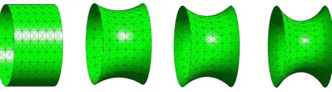
Figure 4. A model (hollow) cylinder
Figure 5. Deformation due to surface tension effect
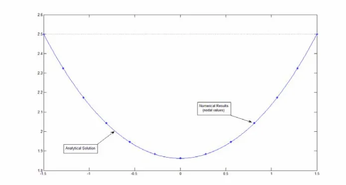
In the limiting case this example amounts to that of finding the minimum surface of he analytical solution of this problem can be attained with recourse to variational r the given dimension, as f x( ) 1.8627 cosh ( / 1.8627) x . The s of such
n revolution. T
calculus, fo proces
deformation is depicted in the figure 5. Furthermore, figure 6 illustrates a comparison betwee the proposed the numerical and analytical result which proves the excellent efficiency of
Figure 6. Numerical vs. Analytical solution
4. Conclusions
A finite element framework for continua with surface potentials has been presented. Based on metry and kinematics of surfaces, the corresponding weak form of the balance equations
unting for contribution geo
acco s from the boundary is derived from the Dirichlet principle of e
Two
hav to confirm the efficiency of the proposed scheme. The solution
Rap
ree-ds
y. minimum potential nergy. A suitable framework for finite element implementation is given.
models for boundary potentials are introduced and corresponding numerical examples e been provided, so as
procedure is robust and shows the asymptotically quadratic rate of convergence for Newton-hson scheme.
References
Adam NK (1941), The physics and chemistry of surfaces. London: Oxford University Press. Adamson E, Gast AP (1997), Physical chemistry of surfaces. Wiley-Interscience.
ellet M (2001), Implementation of surface tension with wall adhesion effects in a th dimensional finite element model for fluid flow. Communications in Numerical Metho in Engineering, Volume 17, Issue 8:563 -- 579.
Ciarlet PG (2006), An Introduction to Differential Geometry with Applications to Elasticit Springer.
Dettmer W, Peric B
D (2006), A computational framework for free surface fluid flows accounting for surface tension. Computer Methods in Applied Mechanics and Engineering, Volume 195, Issues 23-24:3038--3071.
Dettmer W, Saksono PH, Peric D (2003), On a finite element formulation for incompressible newtonian fluid flows on moving domains in the presence of surface tension. Communications in Numerical Methods in Engineering, Volume 19, Issue 9:659 -- 668. Fischer FD, Waitz T, Vollath D, Simha NK (2008), On the role of surface energy and surface
Gibbs JW (1906), The scientific papers of J. Williard Gibbs. Vol. 1: Thermodynamics. New York and Bombay: Longmans, Green, and Co.
Gurtin ME (1975), A continuum theory for elastic material surfaces. Archive for Rational Mechanics and Analysis, 112:97--160.
of
ua with boundary energies. Part I: The two-dimensional case. Computer Methods in Applied Mechanics and
Kuhl E, Askes H, Steinmann P (2004), An ale formulation based on spatial and material settings ethods in 2.
89), The effect of surface stress on crystal-melt and crystal-crystal tallurgica, 37:3119--3138.
Lifshitz EM, Landau LD (1987), Fluid Mechanics, Second Edition: Volume 6 (Course of
Saks
Sim
Gurtin ME, Murdoch A (1975), A continuum theory of elastic material surfaces. Archive Rational Mechanics and Analysis, 57, 291—323.
Javili A, Steinmann P (2009), A finite element framework for contin
Engineering, 198, 27-29: 2198—2208.
of continuum mechanics. part 1: Generic hyperelastic formulation. Computer M Applied Mechanics and Engineering, 193:4207--422
Leo PH, Sekerka RF (19 equilibrium. Acta me
Theoretical Physics). Butterworth-Heinemann.
, Hughes TJR (1994), Mathematical Foundations of Elasticity. Dover Publications. Navti SE, Ravindran K, Taylor C, Lewis RW (1997), Finite element modelling of surface
uids. Computational Mechanics, Volume 14, Number 2:140—153.
ha NK and Bhattacharya K (2000), Kinetics of phase boundaries with edges and junctio Marsden JE
tension effects using a lagrangian-eulerian kinematic description. Computer Methods in Applied Mechanics and Engineering, 147:41--60.
Olson L, Kock E (1994), A variational approach for modelling surface tension effects in inviscid fl
ono PH, Peric D (2006a), On finite element modelling of surface tension. Variational formulation and applications-Part I: Quasistatic problems. Computational Mechanics, Volume 38, 265--281.
Saksono PH, Peric D (2006b), On finite element modelling of surface tension. Variational formulation and applications-Part II: Dynamic problems. Computational Mechanics, Volume 38, 251--263.
ns in a three-dimensional multiphase body. Journal of Mech Phys Solids, 48:2619--41. Steinmann P, Häsner O (2005), On material interfaces in thermomechanical solids. Archive of
Applied Mechanics, 75:31--41.
Steinmann P (2008), On boundary potential energies in deformational and configurational mechanics. Journal of Mechanics and Physics of Solids, 56, 3:772--800.
Zienkiewicz OC, Taylor RL (2005), The Finite Element Method for Solid and Structural Mechanics.