Forecasting secular variation using core flows
Ciar´an Beggan1and Kathy Whaler2
1British Geological Survey, Murchison House, West Mains Road, Edinburgh, EH9 3LA, United Kingdom 2School of GeoSciences, University of Edinburgh, West Mains Road, Edinburgh, EH9 3JW, United Kingdom
(Received November 30, 2009; Revised May 11, 2010; Accepted July 1, 2010; Online published December 31, 2010)
Over the past ten years satellite measurements in combination with data from ground-based observatories have allowed very detailed models of the secular variation (SV) of the Earth’s magnetic field to be constructed. However, forecasting the change of the main field still remains a challenge, primarily because the core processes controlling SV are not sufficiently well understood. Hence, most forecasts do not appeal to any physical modelling constraints but use, for example, polynomial extrapolation from previous measurements. We attempt to apply a physical model to forecast the average SV during 2010–2015 by developing a core flow model. This steady flow model, derived from SV data during 2004.5 to 2009.5, generates a set of Gauss SV coefficients which are used to advect the large scale magnetic field forwards in time. Although this model has not been submitted as a candidate for IGRF-11, we present our SV prediction model and compare it to other candidate IGRF-11 SV models. In addition, we examine the use of the Ensemble Kalman filter to optimally assimilate field models derived from (1) forecast methods and (2) noisy data measurements. Such a scenario might conceivably arise if high quality satellite data with global coverage are not available for a significant period of time. We show that the overall misfit of the assimilated model to the actual field can be lower than the individual misfits of the input models, provided the uncertainties of each model are reasonably well known.
Key words:Magnetic field, secular variation, forecasting, core flows.
1.
Introduction
Forecasting of magnetic field change has been attempted in many forms over the past 300 years since Halley’s ob-servation of westward motion of the agonic line in the At-lantic hemisphere (Halley, 1692). Currently, a widely used forecast of the average secular variation (SV) is produced for the International Geomagnetic Reference Field (IGRF) model every five years. The IGRF models are an agreed set of field coefficients representing snapshots of the mag-netic field at defined times and a set of coefficients fore-casting the average SV for a period of five years into the future. The tenth generation of the International Geomag-netic Reference Field model (IGRF-10) covered the period from 2005.0 to 2010.0 (Macmillan and Maus, 2005). For the IGRF-10 SV model, the methods to estimate the aver-age SV over its five year lifetime used a combination of polynomial extrapolation of satellite data and linear predic-tion filters applied to observatory data. However, these ap-proaches do not invoke any particular physical arguments to support the assumption that the field coefficients will con-tinue to change linearly (which, of course, they do not). Lowes (2000) succinctly outlines the issues faced in fore-casting of SV, noting that an understanding of the fluid pro-cesses within the core might be useful in producing more accurate predictions. Since 2005, a number of forecast-ing techniques have been developed to incorporate phys-ical approximations. For example, Sun et al.(2007) and Fournieret al.(2007) both outline frameworks in which
ob-Copyright cNERC, 2010. All Rights Reserved.
doi:10.5047/eps.2010.07.004
served magnetic field data can be assimilated into physical magnetohydrodynamic models. More recently, Kuanget al.
(2009) have assimilated historical field data into numerical dynamo models to investigate if improvements can be made to forecast field models.
We present a forecast based upon a steady core flow model generated from satellite magnetic data measured over the period 2004.5–2009.5. The SV coefficients derived from a flow model are used to advect the main field Gauss coefficients forwards in time. In Section 2 we examine how well the IGRF-10 SV model forecast has performed while in Section 3 we compare the forecast from a steady flow model over a five year period starting in 2004.5 to the IGRF-10 estimate for 2009.5.
In Section 4, we investigate a method known as the Ensemble Kalman Filter to assimilate field models derived from magnetic measurements (from observatories or satel-lite) and field models computed from a forecast. Ensemble techniques to examine variability and error in geomagnetic studies have previously been applied to core flow modelling by Gillet et al. (2009). We outline our implementation scheme and use error estimates from comparisons to past IGRF and Definitive Geomagnetic Reference Field (DGRF) models to determine reasonable variances for the filter and to illustrate the potential benefits for forecasting in the ab-sense of high-quality satellite magnetic data.
2.
Forecasting Ability
models (Finlayet al., 2010). The models are compared us-ing a root mean square (RMS) difference (or misfit) metric (√d P) calculated by Mauset al.(2008):
n}are the Gauss coefficients of the field and are used to represent bothgmn andh
m
n. The maximum degree of the models isn=m=13 for the main field andn =m=8 (givingdP˙fromg˙mn) for the SV.
The IGRF-10 model coefficients for 2005.0 were gener-ated by forward extrapolation of data measured up to mid-2004 and are a combination of three candidate field models (Mauset al., 2005). Hence a revision is required to produce a retrospective DGRF model for 2005.0. The RMS differ-ence between the IGRF-10 model and the DGRF model for 2005 is approximately 13 nT. The misfit of the IGRF-10 model coefficients to the best available estimate of the in-ternal magnetic field is thus slightly larger than the 5 nT suggested in Mauset al.(2005).
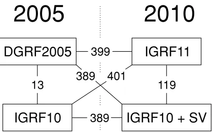
The change in the magnetic field over five years can be estimated by examining the RMS difference between the IGRF-11 model for 2010 and the DGRF model for 2005; it is 399 nT. By comparison, the difference between the IGRF-11 model for 2010 and the IGRF-10 model for 2005 is 401 nT. However, although the IGRF-10 field model ben-efitted from greatly improved availability of satellite data compared to previous IGRF models, the predicted SV co-efficients were still relatively poor and did not accurately forecast the actual SV from 2005 to 2010. The RMS dif-ference between the field for 2010 as estimated from the IGRF-10 model (i.e. IGRF-10 in 2005 plus the sum of the predicted annual SV for five years) and the IGRF-11 model is 119 nT. This is an average RMS misfit of about 24 nT/yr, which is slightly larger than the error estimate of 20 nT/yr given in Mauset al.(2005). Figure 1 summarises the RMS difference relationships.
It can be concluded that adequate techniques to accu-rately estimate the global SV over five years have not yet been developed. This is due, primarily, to the unknown changes of fluid flow within the core (e.g. Holme, 2007). In the next section, we attempt to improve upon the SV forecast by use of a steady core flow model to advect the magnetic field model forward in time.
DGRF2005
Fig. 1. Root Mean Square differences between field models (in nT) for 2005 and 2010.
3.
Flow Modelling
We investigate whether using a core flow model to predict SV can reduce the RMS difference between the actual and predicted field at the end of five years. A study by Mauset al.(2008) examined how well hindcasting of the magnetic field using core flow models reproduced the observed field over 13 years. They employed the ‘frozen flux’ approxima-tion in which diffusion of the magnetic field on large scales is assumed to be negligible on short timescales (Roberts and Scott, 1965). Mauset al.(2008) compared the prediction of the field back in time from the SV generated by a number of core flow modelling assumptions including steady, toroidal only and accelerated flows. They concluded that a steady flow produces the best average fit over a ten-year period. Following on from this result, Beggan and Whaler (2009) investigated how well a steady flow generated from satel-lite data could predict secular variation. Using the same techniques, here we test how well a steady core flow model developed from CHAMP satellite data from 2001.4–2004.5 can predict the change in the magnetic main field between 2004.5 and 2009.5. These time periods are covered by cur-rent satellite field models and allow consistent comparisons to be made.
For this study, we prepared a series of 27 monthly SV data sets, over the period 2001.4–2004.5, generated from CHAMP satellite data using the ‘Virtual Observatory’ (VO) method of Mandea and Olsen (2006). The SV data were inverted for toroidal and poloidal flow using the linear re-lationship between SV and flow spherical harmonic coef-ficients. The relation is through the Gaunt/Elsasser matrix (H) whose elements depend on the main field coefficients which change with time (Whaler, 1986). The main field, SV and flow coefficients are truncated at degree and order
nmax=14, and thus we have assumed that only large scale
flows are responsible for the large scale SV. We assumed a steady flow model, with tangential geostrophy (Hills, 1979; Le Mou¨el, 1984) imposed as a weak penalty norm con-straint. The Gauss coefficients (in the vectorg) from the POMME3 main field model (Mauset al., 2006) were used in the flow inversion.
Employing the method outlined in Beggan and Whaler (2009), the steady flow model coefficients (mˆSF) were used
to forecast the change in the magnetic field over the five year period from 2004.5 to 2009.5. This period was cho-sen to allow direct comparison between the forecast field model coefficients and the CHAOS-2s model (Olsenet al., 2009). Thus the Gauss coefficients from CHAOS-2 (up to degree 12) for 2004.5 were used as the starting field model. The field was advected forward (forecast) over successive months (t) for five years (until 2009.5) using the equation:
gt+1=gt+(HtmˆSF)/12 (2)
with the Ht matrix updated at every timestep using the main field coefficients forecast from the previous timestep, making the system slightly non-linear.
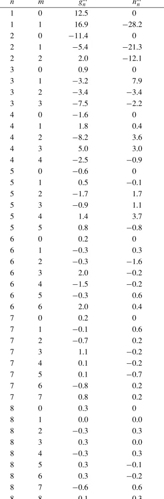
Table 1. Predicted average SV coefficients from the steady flow model, up to degree and order 8.
n m gnm hmn
the starting point. The misfit of the IGRF-10 SV model at 2009.5 to the CHAOS-2 model was 102 nT.
We verified that the flow model generated directly from the SV derived from the VO method is insensitive to the main field model used in the inversion by comparing the prediction of a steady flow derived from the CHAOS main field model (Olsenet al., 2006) instead of POMME3. The resulting flow model was only slightly different from that derived from the POMME3 model, and the RMS differ-ence between the SV forecast model using the CHAOS-derived steady flow after five years was also approximately 85 nT. Thus, SV estimates from steady core flows give a
lower RMS misfit over five years and suggest a forecasting method employing core flow modelling may be beneficial.
We applied the same methodology to forecast the aver-age SV over the period 2010–2015, now based on a steady flow derived from a longer time-series of fifty monthly VO SV models using CHAMP data from 2004.5–2009.5. Due to changes in core flows associated with geomagnetic jerks (e.g. Gubbins, 1984; Wardinksiet al., 2008), we use satel-lite data after the jerk in about 2003.4 (Olsen and Mandea, 2007). The field was computed using Eq. (2), starting with the main field coefficients for 2009.5 from CHAOS-2. The coefficients of the average SV (given in Table 1) were cal-culated by dividing the difference between the main field coefficients predicted at 2010 and those forecast at 2015 by five years.
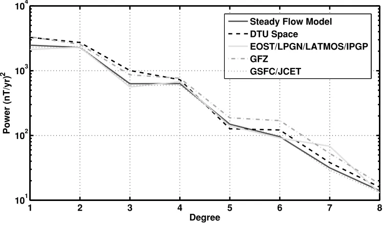
Figure 2 shows the Lowes-Mauersberger spectrum of the SV derived from the steady flow model for 2009.5– 2014.5, compared to those of IGRF-11 candidate models A (DTU), E (EOST/ LPGN/ LATMOS/ IPGP), G (GFZ) and H (GFSC/JCET) illustrating that the SV prediction of the steady flow model is within the range of these proposed models. It also lies within the range of the other four can-didates which are not shown to avoid cluttering the figure. The prediction of candidate Model A has more power in the lower degrees (n =1–4), while Model E and Model H predictions are very similar for degreesn=2–6.
4.
Data Assimilation
We wish to investigate whether it is possible to combine a relatively good forecast field model with a lower qual-ity ‘measured’ field model to improve the estimate of the actual field. For example, if the existing set of satellites fail before Swarm is fully operational, there could be a gap in which our present high-quality global coverage is di-minished and we may become mostly reliant upon ground-based observatories and repeat stations to produce global magnetic field models. Due to the uneven geographic dis-tribution of ground-based observations these models have much higher uncertainties than models employing satellite data. This section looks at a potential method for mitigat-ing the impact of such an event by employmitigat-ing an optimal data assimilation algorithm to make best use of all available information. We investigate whether a sufficiently accu-rate forecast can be obtained using an initial high-resolution satellite field model, combined with a flow model for advec-tion of the field and intermittent updates from a simulated lower quality ground-based field model.
1 2 3 4 5 6 7 8 101
102 103 104
Power (nT/yr)
2
Degree
Steady Flow Model DTU Space
EOST/LPGN/LATMOS/IPGP GFZ
GSFC/JCET
Fig. 2. Spectrum of the Steady Flow model SV prediction for 2010–2015 compared to that of the IGRF-11 SV candidate Models A (DTU Space), E (EOST/LPGN/LATMOS/IPGP), G (GFZ) and H (GFSC/JCET).
4.1 Ensemble Kalman filtering
A traditional single-state Kalman Filter is implemented in two steps: (1) prediction of the evolution of the model state by equations believed to adequately represent the sys-tem and (2) assimilation of a measurement to correct any accumulated error from the model (Kalman, 1960). The ad-vantage of the Kalman filter is that measurements can be assimilated whenever they are available. When no data are available, the process is modelled by forecasting. Even rel-atively poor data can be used to constrain the forecast, as they are optimally included into the filter. At a timet, the optimal blending of a forecast (xf
t) and measurement (zt) to generate the assimilated state vector, xat, is through the so-called Kalman gain matrix (Kt):
xat =xft+Ktzt−xft (3)
with
Kt=Pft
Pft+Q
−1
, (4)
wherePf
tis the error covariance matrix of the model equa-tions andQis the error covariance matrix for the measure-ment.
In our application of this method, we setxf
tto be a vector of Gauss coefficients produced from a forecast as defined in Eq. (2). If a field model, derived from observed data, becomes available it can be represented aszt, another vector of Gauss coefficients. Combining the measurement and the forecast depends on how the errors for each vector are defined, which we will discuss in Section 4.2.
Examination of Eqs. (3) and (4) reveals some important aspects of the filter. If the measurementzt and model pre-dictionxf
t are equal, then the update has no effect. If the elements of the measurement covariance error matrix (Q) are small, then(zt−xft)is more heavily weighted in the
up-date. Equally, if the model covariance error matrix elements (Pf) are small then the forecast state (xf
t) is more important. The balance between these matrices (i.e. the estimated
un-certainties of the model and measurement) controls the as-similation step.
The Kalman Filter was designed as a linear filter. In a non-linear regime, it can become unwieldy and unreliable. To overcome such limitations, Evensen (1994) suggested an algorithm for data assimilation employing Monte Carlo methods as an alternative. The state of a process at any particular time is represented as a vector inr-dimensional space, where r is the number of parameters in the sys-tem. In an Ensemble Kalman Filter the uncertainty of our knowledge of the process is represented by perturbing the inputs to the model forecast equations randomly by a known variance (with zero-mean) to produce an ‘ensemble’ of states—conceptually imagined as a ‘cloud’ of points inr -dimensional space. The evolution of the states though time is controlled by propagating the entire ensemble forward using model equations of the system behaviour. In essence, this is nominally equivalent to running many instances of the Kalman Filter in parallel.
When an ‘observation’ is available, it can be optimally assimilated into the ensemble by applying the standard Kalman Filter equations. With a sufficiently large ensem-ble (determined through experimentation), the mean state should represent the maximum likelihood value for the pro-cess at the time. The evolution of the ensemble can be explored by examining the ‘spread’ of the states about the mean.
1 2 3 4 5 6 7 8 9 10 11 12 0
10 20 30 40 50 60
Degree
RMS difference (nT)
Steady Flow Model (2009.5) IGRF10 SV Model (2009.5)
EnKF Uncertainty Model I EnKF Uncertainty Model II EnKF Uncertainty Model III
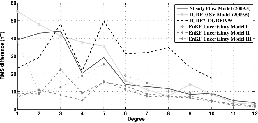
Fig. 3. Root Mean Square difference per degree (defined in Eq. (5)) to the CHAOS-2 model (at 2009.5) of the field predicted by the IGRF-10 SV model, the Steady Flow SV model and three EnKF simulations with different errors assumptions as discussed in Section 4.3. Also shown is the RMS difference per degree between the IGRF-7 and DGRF field models for 1995.0. See text for details.
than 500 is adequate.
The ensemble is initiated by perturbing the Gauss coef-ficients of the CHAOS-2 field model in 2004.5. The ini-tial perturbation to thegm
n field coefficients is based on an estimate of the standard deviation for each coefficient, dis-cussed in detail in the next section. A matrix of normally distributed random numbersN(0,1)is generated, which is then multiplied by the standard deviation of the flow co-efficients to give a perturbed flow coefficient matrix. This perturbed flow coefficient matrix is pre-multiplied by the Hmatrix to produce a matrix of perturbed SV coefficients, correctly scaled to reflect the uncertainty in the flow mod-els. The perturbed SV coefficient matrix is then added to the initial state vector to produce the initial ensemble matrix. Once this initial ensemble has been created, forecasting and assimilation can take place.
The forecast (prediction) of the field is driven forwards by the summation of (1) the field coefficients and (2) the monthly SV coefficients from the flow model. In addition, at each timestep, model noise is added to simulate the vari-ance of the ensemble, forcing it to grow at each forecast iteration. These steps are repeated until a measurement be-comes available for assimilation into the ensemble.
Over time, the forecast field will begin to diverge from the actual field. To improve the forecast, data can be input into the ensemble to update (correct) it. The data have as-sociated errors which are used to generate a perturbed data ensemble. Data, for example a set of Gauss coefficients (zk) with a certain (estimated or known) error are available. A matrix of zero-mean Gaussian random numbers is gener-ated and scaled with the data error. The data are then added to the matrix of scaled random numbers to produce a ma-trix of ‘perturbed data’. Using Eq. (3) this data perturba-tion matrix and the perturbed SV coefficients are optimally assimilated into the ensemble at this timestep. The covari-ance matrices (PandQ) can be estimated from the ensem-ble and measurement errors (Evensen, 1994). In this study
we assimilate low quality (i.e. large assumed variance; see Section 4.3) Gauss coefficients of the CHAOS-2 field model into the ensemble via thezkterm.
4.2 Uncertainty estimation
The determination of realistic uncertainties to apply to the model coefficients of the field and the SV from the flow is difficult. For a Kalman Filter to be optimal it is important that the uncertainty estimate of the forecast field generated by the flow model and the uncertainty of the ‘measured’ field model should be similar in magnitude. If one has a much lower uncertainty estimate than the other, then it tends to dominate the filter.
One approach to estimating the uncertainty is to examine which field coefficients have in the past been most poorly predicted at the end of a five year period. As noted in Section 3, the field model prediction from 2004.5 to 2009.5 of the IGRF-10 SV model has a RMS difference of approxi-mately 102 nT, while the RMS difference of the steady flow model prediction is 85 nT. We can investigate the difference in more detail by defining the RMS difference per degree (√d Pn) as:
d Pn= n
m=0
(n+1)(gnm)Model A−(gnm)Model B
2
(5)
Figure 3 shows the RMS difference per degree to the CHAOS-2 model (in 2009.5) of the IGRF-10 SV predic-tion for five years and the steady flow model SV predicpredic-tion. The RMS difference per degree shows that the field model forecast by the IGRF-10 SV prediction (grey solid line, cir-cle marker) differs strongly from the CHAOS-2 model at degrees 1–5. In contrast, the field model forecast by the steady flow model (black solid line) is poorest at degree 3 (coefficientsh3
3andh13), but better at degrees 1, 2 and 4–6.
between satellite field models and models derived from ground-based measurements arise, we examined the differ-ence between IGRF-7 model (valid 1995–2000) coefficients as defined for 1995 and the DGRF model for 1995 from Chambodutet al.(2005). The DGRF model was calculated from the backward projection of high quality satellite data from 2000 onwards, though it should be noted that the back-propagation is imperfect. The RMS difference between the IGRF-7 model and the revised DGRF is 104 nT (up to de-gree 10) and we have plotted the RMS difference per dede-gree between models in Fig. 3 (dashed black line), again up to degree 10. The IGRF-7 model is relatively good at degrees 1, 2 and 4 but poorer at degrees 3 and 5. Whether this pat-tern is peculiar to the IGRF-7 model or applies in general to field models derived mainly from ground-based data is not known.
We can now use the absolute differences of the Gauss co-efficients between the IGRF-7 and DGRF models (dashed black line) as reasonable estimates for the noise pertuba-tions to apply to an assimilated ‘measurement’ within the EnKF. Similarly, the differences in the Gauss coefficients between the field forecast by the SV from the steady flow model and CHAOS-2 (solid black line) can be used as es-timates for the variance of the forecast. The absolute dif-ferences are relatively similar in magnitude and somewhat complementary—the errors of the IGRF-7 field model are lower at degree 1 and 2 and similar for degree 3 and 4, while the errors of the flow model SV forecast are lower at degrees 5–12. As the IGRF-7 errors only extend to degree 10, the errors for coefficients of degrees 11 and 12 were set to a value of 0.5 nT. (This is the median of the absolute value of the degree 11 and 12 coefficients of IGRF-10).
In the EnKF, random perturbations to the ensemble states can now be controlled using the absolute differences be-tween the coefficients of IGRF-7 and DGRF for 1995 as the expected standard deviations. Each state coefficient (or Gauss coefficient for this study i.e.xf
t) perturbation is thus drawn from a normal distributionN(0,1)and scaled by the respective error. We explore the effect of using three differ-ent uncertainty assumptions for the ‘measured’ field model input to the filter.
4.3 EnKF simulation results
A steady flow model (with a tangential geostrophic con-straint) was generated from SV data over the period 2001.4– 2004.5. The CHAOS-2 model for 2004.5 was used as the starting point for the EnKF field ensemble with each en-semble state propagated forward with a timestep equal to one-twelveth of a year using a set of perturbed SV coef-ficients from the steady flow model. The ensemble states were forecast forward in time using:
grt+1=grt +(HtmˆSF)+N(0,1)rt ∗σ m n
/12 (6)
wheregrt are the Gauss coefficients of ensemble stater at timestept. The values ofσnmare the estimated uncertainties, up to degree and ordern = m = 12, computed from the difference between the steady flow model prediction and the CHAOS-2 model at 2009.5.
At every twelfth timestep (i.e. annually), a set of noisy Gauss coefficients was assimilated into the system using Eqs. (3) and (4). The Gauss coefficients, initally generated
from the CHAOS-2 model, have Gaussian noise added with a standard deviation derived from the RMS difference of the IGRF-7 and DGRF1995 models to simulate the expected uncertainty of a ground-based field model. The results of three different uncertainty assumptions for the assimilated field model were tested. (Note, the EnKF uncertainty mod-els are given roman numerals to avoid confusion with the IGRF-11 candidate models).
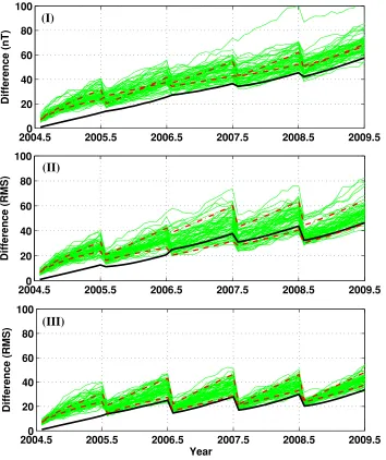
Figure 4 shows the RMS difference between the CHAOS-2 model and three Ensemble Kalman Filter noise simulations. In each panel, the thin green lines represent the evolution of 1000 individual field model ensemble states over 61 months. The solid black line represents the mean of the ensemble states, the dashed line is the+1σ field model and the dot-dashed line is the−1σ field model (computed from the mean of the ensemble). In the upper panel, uncer-tainty model I, the forecast model and ‘measurement’ field model errors are similar in magnitude. The mean RMS dif-ference at 2009.5 is 58 nT. Figure 4 (upper panel, I) illus-trates the spread of the ensemble states but shows that the mean of the ensemble is the best fit model overall (though two of the ensemble states do have a slightly lower misfit at 2009.5). The RMS difference per degree of the mean of the ensemble to the CHAOS-2 model is shown in Fig. 3 (dotted red line, diamond marker). The overall difference per degree is, on average, smaller at 2009.5 than either of the input errors (from the IGRF-7 minus DGRF1995 model or the CHAOS-2 model minus the Steady Flow model at 2009.5). This illustrates one of the strengths of a Kalman filter—the assimilation of ‘forecast’ and ‘measurement’ can improve upon both, by optimally combining the best parts of each, provided the uncertainties are reasonably compli-mentary.
We investigated the outcome of using better field mod-els in the assimilation by reducing the noise added to the CHAOS-2 field coefficients. In uncertainty model II, the ‘measured’ field model errors were sampled from a distri-bution with spread approximately half as large as the field model errors in I (i.e. the standard deviations were divided by 2). The RMS difference to the CHAOS-2 model in 2009.5 is 47 nT. In uncertainty model III the field model errors are approximately a quarter the size of the model er-rors in I, with RMS difference to CHAOS-2 in 2009.5 of 34 nT. Thus, as the field model improves, the RMS dif-ference becomes smaller, as would be expected. The RMS difference per degree for models II and III are also shown in Fig. 3 (dashed red line and dash-dot red line with dia-mond markers, respectively). Due to the random nature of the added noise, some degrees are better fit than others. For example, degree 3 is better fit in model I than model II, de-spite the average uncertainty being smaller for the latter. At higher degrees (n =11 and 12), the difference of all the models to the CHAOS-2 model is roughly equal.
2004.50 2005.5 2006.5 2007.5 2008.5 2009.5 20
40 60 80 100
Difference (nT)
2004.50 2005.5 2006.5 2007.5 2008.5 2009.5
20 40 60 80 100
Year
Difference (RMS)
2004.50 2005.5 2006.5 2007.5 2008.5 2009.5
20 40 60 80 100
Difference (RMS)
(II)
(I)
(III)
Fig. 4. Root Mean Square difference to the CHAOS-2 model of three Ensemble Kalman Filter simulations. The thin green lines represent the evolution of 1000 individual field model ensemble states over 61 months. The solid black line represents the mean of the ensemble states, the (lower red) dashed line is the+1σfield model and the (upper red) dot-dashed line is the−1σfield model as calculated from the mean of the ensemble. Model I assumes that the forecast model uncertainties and the assimilated field model uncertainties are set to be approximately similar in magnitude. Model II has assimilated field model uncertainties that are approximately one-half the size of model I. The assimilated field model uncertainties for model III are approximately one-quarter the size of those in model I.
5.
Conclusions
The RMS difference between the IGRF-10 SV predic-tion for 2009.5 starting from a model of the field for 2004.5 is estimated to be approximately 102 nT. Thus, the aver-age annual RMS misfit between the IGRF-10 model and the ‘true’ magnetic field was about 21 nT. Using a steady flow model generated from SV data prior to 2004.5 to pre-dict the SV for a similar period of time (2004.5–2009.5) resulted in an average RMS difference of approximately 17 nT/yr. This suggests improvement in the SV prediction may be possible. While there is a large variation between proposed IGRF-11 SV candidate models, the coefficients derived from the steady flow model are within the range of most of the candidate models, indicating it is not an unrea-sonable estimate.
The RMS difference between the DGRF1995 field model (derived from the backward projection of satellite data) and
the IGRF-7 model for 1995 (derived primarily from ground-based observatories) is 104 nT. In a future scenario where only a relatively poor field model is available, we show that it is possible to improve the prediction using data assimila-tion with a field model derived from a steady core flow fore-cast. If a high-quality starting field model is available with only lower-quality updates, then the combination of fore-casts from a core flow model and lower quality field models using an Ensemble Kalman filter can reduce the RMS er-rors of the resulting forecast. The potential improvements are strongly dependent on the relative uncertainties of each model.
Acknowledgments. We would like to thank Susan Macmillan
part of the NERC GEOSPACE programme, funded under grant NER/O/S/2003/00674. This paper is published with the permis-sion of the Executive Director of the British Geological Survey (NERC).
References
Beggan, C. D. and K. Whaler, Forecasting change of the magnetic field using core surface flows and ensemble Kalman filtering,Geophys. Res. Lett.,36, L18303, 2009.
Chambodut, A., B. Langlais, and M. Mandea, Candidate main-field models for the Definitive Geomagnetic Reference Field 1995.0 and 2000.0,
Earth Planets Space,57, 1197–2002, 2005.
Evensen, G., Sequential data assimilation with a nonlinear quasi-geostrophic model using Monte Carlo methods to forecast error statis-tics,J. Geophys. Res.,99, 10,143–10,162, 1994.
Finlay, C. C., S. Maus, C. D. Beggan, M. Hamoudi, F. J. Lowes, N. Olsen, and E. Th´ebault, Evaluation of candidate geomagnetic field models for IGRF-11,Earth Planets Space,62, this issue, 787–804, 2010. Fournier, A., C. Eymin, and T. Alboussiere, A case for variational
geomag-netic data assimilation: insights from a one-dimensional, nonlinear, and sparsely observed MHD system,Nonlin. Proc. Geophys.,14, 163–180, 2007.
Gillet, N., A. Pais, and D. Jault, Ensemble inversion of time-dependent core flow models,Geochem. Geophys. Geosyst.,10, Q06004, 2009. Gubbins, D., Geomagnetic field analysis—II. Secular variation consistent
with a perfectly conducting core,Geophys. J. R. Astron. Soc.,77, 753– 766, 1984.
Halley, E., On the cause of the change in the variation of the magnetic needle; with an hypothesis of the structure of the internal parts of the Earth,Phil. Trans. R. Soc. Lond.,17, 470–478, 1692.
Hills, R., Convection in the Earth’s mantle due to viscous shear at the core-mantle interface and due to large-scale bouyancy, Ph.D. thesis, N. M. State Univ., Las Cruces, 1979.
Holme, R., Large scale flow in the core, inTreatise on Geophysics, Vol. 8, 107–130, Elsevier, 2007.
Kalman, R., A new approach to linear filtering and prediction problems,
Trans. ASME J. Basic Eng.,82, 35–45, 1960.
Kuang, W., A. Tangborn, Z. Wei, and T. Sabaka, Constraining a numerical geodynamo model with 100 years of surface observations,Geophys. J. Int.,179, 1458–1468, 2009.
Le Mou¨el, J.-L., Outer-core geostrophic flow and secular variation of
Earth’s geomagnetic field,Nature,311, 734–735, 1984.
Lowes, F. J., An estimate of the errors of the IGRF/DGRF fields 1945– 2000,Earth Planets Space,52, 1207–1211, 2000.
Macmillan, S. and S. Maus, International Geomagnetic Reference Field— the tenth generation,Earth Planets Space,57, 1135–1140, 2005. Mandea, M. and N. Olsen, A new approach to directly determine the
secular variation from magnetic satellite observations,Geophys. Res. Lett.,33, L15306, 2006.
Maus, S., S. Macmillan, F. Lowes, and T. Bondar, Evaluation of candi-date geomagnetic field models for the 10th generation of IGRF,Earth Planets Space,57, 1173–1181, 2005.
Maus, S., M. Rother, C. Stolle, W. Mai, S. Choi, H. L¨uhr, D. Cooke, and C. Roth, Third generation of the Potsdam Magnetic Model of the Earth (POMME),Geochem. Geophys. Geosyst.,7, Q07008, 2006.
Maus, S., L. Silva, and G. Hulot, Can core-surface flow models be used to improve the forecast of the Earth’s main magnetic field?,J. Geophys. Res.,113, B08102, 2008.
Olsen, N. and M. Mandea, Investigation of a secular variation impulse using satellite data: the 2003 geomagnetic jerk,Earth Planet. Sci. Lett., 255, 94–105, 2007.
Olsen, N., H. L¨uhr, T. Sabaka, M. Mandea, M. Rother, and L. Toffner-Clausen, CHAOS: a model of the Earth’s magnetic field derived from CHAMP, Oersted, and SAC-C magnetic satellite data,Geophys. J. Int., 166, 67–75, 2006.
Olsen, N., M. Mandea, T. J. Sabaka, and L. Tøffner-Clausen, CHAOS-2—a geomagnetic field model derived from one decade of continuous satellite data,Geophys. J. Int.,179, 1477–1487, 2009.
Roberts, P. and S. Scott, On the analysis of the secular variation. 1. A hydromagnetic constraint: Theory,J. Geomag. Geoelectr.,17, 137–151, 1965.
Sun, Z., A. Tangborn, and W. Kuang, Data assimilation in a sparsely ob-served one-dimensional modeled MHD system,Nonlin. Proc. Geophys., 14, 181–192, 2007.
Wardinski, I., R. Holme, S. Asari, and M. Mandea, The 2003 geomagnetic jerk and its relation to the core surface flows,Earth Planet. Sci. Lett., 267, 468–481, 2008.
Whaler, K., Geomagnetic evidence for fluid upwelling at the core-mantle boundary,Geophys. J. R. Astron. Soc.,86, 563–588, 1986.