R E S E A R C H
Open Access
Some advanced parametric methods for
assessing waveform distortion in a smart grid
with renewable generation
Luisa Alfieri
Abstract
Power quality (PQ) disturbances are becoming an important issue in smart grids (SGs) due to the significant economic consequences that they can generate on sensible loads. However, SGs include several distributed energy resources (DERs) that can be interconnected to the grid with static converters, which lead to a reduction of the PQ levels. Among DERs, wind turbines and photovoltaic systems are expected to be used extensively due to the forecasted reduction in investment costs and other economic incentives. These systems can introduce significant time-varying voltage and current waveform distortions that require advanced spectral analysis methods to be used. This paper provides an application of advanced parametric methods for assessing waveform distortions in SGs with dispersed generation. In particular, the Standard International Electrotechnical Committee (IEC) method, some parametric methods (such as Prony and Estimation of Signal Parameters by Rotational Invariance Technique (ESPRIT)), and some hybrid methods are critically compared on the basis of their accuracy and the computational effort required.
Keywords:Smart grid; Dispersed generation; Power quality; Waveform distortion; DFT; Parametric methods
1 Introduction
Currently, significant modifications are taking place in distribution systems as they move toward the future use of smart grids (SGs). The main objectives of SGs are the efficient use of energy, the reduction of losses in the sys-tem, improvement in the power quality (PQ), and to en-courage the use of distributed generation, in particular renewable energy sources [1-4]. In this context, the in-creasing use of controllable and non-linear loads and the new needs of liberalized markets impose new PQ re-quirements in order to avoid dangerous effects [5-7].
Among the disturbances mentioned above, the distor-tions of the voltage and current waveforms are of great interest, and they have been discussed extensively in the literature. Both types of distortions are due mainly to the extensive use of electronic power converters to sup-ply loads and to connect dispersed generation (DG) units or electrical storage systems to the grid.
Photovoltaic systems (PVSs) and wind turbine systems (WTSs) are the fastest growing systems for meeting the
requirements of dispersed generation. Their growth is due to the expected cost reduction and to active govern-ment policies in many countries that have encouraged their use in power grids in the last few decades. These DG units can be interfaced to the grid through either partially rated power converters or full-scale power elec-tronic devices that can inject harmonic currents that cause voltage distortions [6-8]. Therefore, there is a pressing need to study the impacts of such DG systems on waveform distortions in distribution networks [9]. Thus, the main objective of this paper is to apply some of the advanced methods for the assessment of the wave-form distortions that are caused by different configura-tions of PVSs and WTSs [10-20].
PVSs and WTSs generate distorted, time-varying wave-forms. As a result, great attention is required to evaluate the PQ indices to acquire information that must be de-duced from the analyses of the spectral components of the waveforms and their locations as a function of time [5,21].
The International Electrotechnical Committee's (IEC) standard recommendations for signal processing use the Discrete Fourier Transform (DFT) over successive, rect-angular time windows with the time duration set to 10 Correspondence:[email protected]
Department of Electrical Engineering and Information Technology, University of Naples Federico II, Via Claudio, 21, 80125 Napoli, Italy
or 12 cycles of the fundamental period for 50-Hz sys-tems or 60-Hz syssys-tems, respectively, to evaluate the spectral components [22,23]. However, even though the standard method can provide a global quantification of the waveform distortion, it has limited ability to obtain more detailed information in the analysis of a single spectral component. This is due to some well-known problems that characterize the DFT, i.e., the spectral leakage that arises when the duration of the time win-dow is not correctly synchronized with the fundamental period of the power system [5].
Many solutions have been proposed in the relevant lit-erature to overcome the spectral leakage problems by using DFT-based methods or parametric methods, such as Prony and Estimation of Signal Parameters by Rota-tional Invariance Technique (ESPRIT) [24-30]. In particu-lar, in [27,28], the Sliding-Window Prony method and the Sliding-Window ESPRIT method were used to provide an accurate estimation of both the harmonic and interhar-monic components with high-frequency resolution, but the computational burden was excessive. Other authors have proposed hybrid methods that include DFT and parametric methods to analyze the different frequency bands of a signal separately to reduce the computational burden and provide acceptable accuracy [29,30].
Recently, some authors [31,32] proposed two new, modified sliding-window parametric methods based on modifications of the Prony and ESPRIT signal models. In fact, these methods are based on the observation of the reduced time variability of the frequencies of the spectral components. Then, the frequency values of the spectral components were assumed to be constant over time, thereby reducing the number of unknown parameters of the signal model and the dimension of related equation systems to be solved.
The main aims of this paper can be summarized as follows:
– To provide a depth application of some methods for the assessment of waveform distortion caused by PVS and WTS generators. In particular, the DFT method, parametric methods (Prony and ESPRIT), hybrid methods, and modified sliding-window parametric methods are presented and critically compared on the basis of the accuracy of the results they produce and their computational burdens, taking into account both test and measured waveforms.
– To explore and compare the theoretical waveform distortions introduced by PVS and WTS
generators and the distortions detected by the considered methods in some current waveforms measured at the point of common coupling of PVS and WTS.
The paper is organized as follows. Section 1.1 de-scribes waveform distortions in detail that result from the different configurations of the PVS and the WTS schemes. In Section 1.2, the Sliding-Window ESPRIT and Prony methods are exposed, and in Section 1.3, de-tailed descriptions of the sliding-window hybrid methods and the sliding-window modified parametric methods are presented. In Section 1.4, we describe several case studies that were based on synthetic and measured waveforms of PVSs and WTSs. This article’s conclusions are given in Section 2, and the DFT method is discussed in Appendix A.
1.1 Waveform distortion in PV systems and WT systems It is well known that solar energy and wind energy cur-rently are the most diffuse sources of renewable energy. The following sub-sections provide an overview of the waveform distortions caused by the most common PVS and WTS configurations. The overview deals with the primary spectral emissions that result from disturbances introduced by the specific nature of the system that is being considered, and it also deals with the secondary spectral emissions that are due to disturbances caused by other sources near the system, such as non-linear loads and power communication signals [18]. Note that the distortions introduced by the PVSs and WTSs gener-ally correspond to spectral components that are included in a wide range of frequencies.
For the sake of clarity, in the following, the spectral components up to 2 kHz are referred as ‘low-frequency components’, and the spectral components over 2 kHz are referred as‘high-frequency components’.
1.1.1 Photovoltaic systems
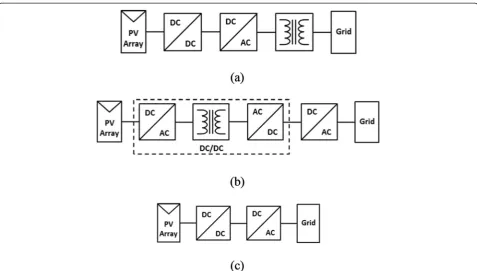
Photovoltaic panels are connected to the grid through an inverter that converts DC to AC and ensures that particular specifications for voltage and frequency are met and that other important tasks are performed, such as maximum power point tracking (MPPT) [10].
Three-phase or single-phase inverters are used, with the former ensuring no zero-sequence emission in the spectra of the waveforms. Multi-string inverters also are available to obtain the combined benefit of the previous configurations [19].
Figure 1 shows the most diffuse topology solutions for the inverters, i.e., (i) inverters with line frequency isolation transformers (Figure 1a), (ii) inverters with high-frequency isolation transformers (Figure 1b), and (iii) inverters with-out isolation transformers (Figure 1c) [10,19].
that increases slightly as the amount of power being pro-duced increases.
Practical experience has indicated that PVSs consti-tuted by multiple inverters produce lower levels of emis-sions than PVSs that have a unique, large-size inverter [20]. The spectral emissions of PVSs at the point of common coupling (PCC) determine both the low- and high-frequency spectral components.
The low-frequency emissions can be due to both back-ground distortion and over-modulation by the inverter. The amplitudes of these low-frequency spectral compo-nents in a single photovoltaic plant are generally charac-terized by a current total harmonic distortion (THDi) smaller than 10%, but in resonance conditions, signifi-cant voltage distortions and problems for the electric network have been documented [19].
The high-frequency emissions basically are due to the PVS inverter and they are specifically due to the pulse-width modulation (PWM) technique that is used. These emissions are always present during the power produc-tion of the system, and they are null when the inverter is turned off; moreover, for the current waveform of a sin-gle photovoltaic plant in ideal operating conditions, the amplitudes of these high-frequency spectral components are higher than those of the low-frequency spectral com-ponents [18,19]. These spectral comcom-ponents depend on the type of inverter and on its switching frequency, and they are mostly harmonics that appear as sidebands that
are centered around integer multiples of the switching frequency [19,33]. Since the switching frequency is gen-erally in a range between 10 and 20 kHz, actually, there still are no adequate and consolidated standards for these high-frequency emissions. Currently, however, the increasing number of spectral components above 2 kHz has resulted in an increased intensity of research activ-ities on this issue [19]. Note that, also at high-frequency, there are often spectral components due to the back-ground voltage, which could become relevant for the series resonance effect.
1.1.2 Wind turbine systems
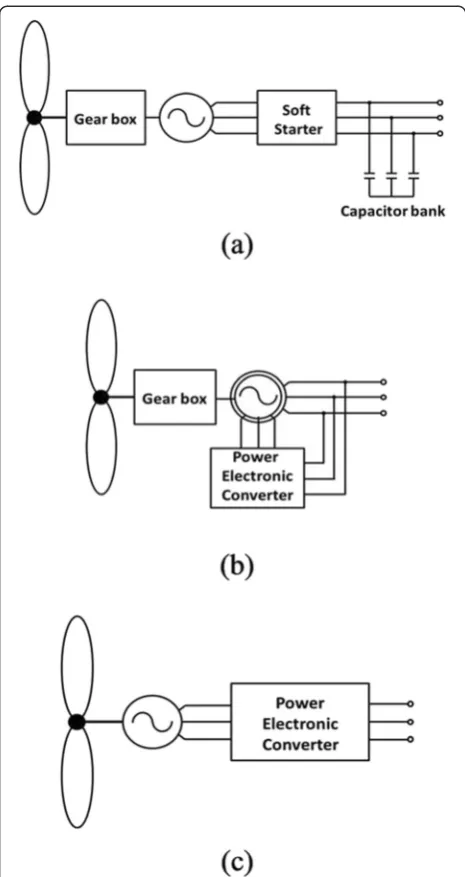
At the current time, the main large wind turbine schemes are (i) the fixed-speed wind turbine system, (ii) the doubly fed induction generator (DFIG), and (iii) the full-converter wind turbine generator [17,34,35]. Figure 2 shows the block schemes of the three configurations.
Figure 2a shows a fixed-speed wind turbine system in which a squirrel-cage induction generator (SCIG) works in a speed-limited range above the synchronous speed. An electronic soft starter generally is provided to avoid the increase of current during the start-up phase. Also, a bank of capacitors is used to compensate for the reactive power.
The spectral emissions of this scheme primarily are caused by the action of the soft starter, which introduces odd harmonic components at low frequency. Triple
components are usually due to voltage unbalances. Gen-erally, for this configuration, the most significant com-ponents detected at the PCC are the 3rd, 5th, 7th, 9th, 11th, and 13th harmonic orders [17].
In a DFIG, the windings of the stator are connected directly to the grid, whereas, on the rotor circuit, there is a back-to-back, partial-scale static converter with a rated power that is roughly equal to 30% of the genera-tor's power.
For this scheme, the spectral emissions in the grid are mainly due to the static converter. Three main types of spectral emissions can arise at the PCC, i.e., (i) inherent components, (ii) switching spectral components, and
(iii) spectral components due to the unbalance condi-tions and/or background voltages [17,36].
The first category includes mostly low-frequency com-ponents, and it is due to a non-sinusoidal air gap flux, which produces distorted voltages and currents at the frequencies fk= |6k(1−s) ± 1|f0,s, with k= 1, 2, …, and
wheres is the generator slip, and f0,sis the fundamental
frequency of the stator voltage. These spectral compo-nents are time-varying with the speed of the DFIG rotor. The spectral components that belong to the second class are due to both the rotor-side and grid-side con-verters and are linked to the PWM technique that was used. They are mostly high-frequency spectral compo-nents, but in over-modulation conditions, low-frequency components also can be detected. Under ideal condi-tions, the aforesaid harmonics and interharmonics are as follows: (i) for the grid side, in correspondence with the frequencies fPWM;k;m g ¼ kfsw;gmf0;s
h i
, withk,m= 1, 2,… and wheref0,sis the nominal frequency of the system, and
fsw,gis the PWM switching frequency on the grid side; (ii)
for the rotor side, in correspondence with the frequencies fPWM;k;m r¼ kfsw;rmf0;r
h i
, withk, m= 1, 2,…and where f0,r=sf0,sis the fundamental frequency of the waveform to
generate for the rotor winding, and fsw,r is the PWM
switching frequency on the rotor side.
Note that the rotor-side converter works at a fre-quency that is linked to the generator slip and that the aforesaid spectral components could be shifted because of the air-gap coupling between the rotor current and the stator circuit [36].
The third type of spectral emissions is the spectral components that are introduced by not-ideal operating conditions and by the WTS's auxiliary, non-linear loads, such as controllers and motors [12,17,36].
Figure 2c shows the full-converter wind-turbine gener-ator scheme, which consists of a permanent-magnet syn-chronous generator connected to the grid by means of a full-scale, power electronic converter with a rated power that is 110% of the generator's power.
Also in this scheme, the emission of spectral compo-nents is caused mainly by the static converter, but unlike the previous case, there is no direct influence on the air-gap flux, so the spectral content of the waveforms at the PCC is less. The most significant components are har-monics of 6k± 1 order (5th, 7th, 11th, 13th,…) at low frequency, typical of a six-pulse, three-phase bridge. How-ever, for the high frequency, the typical spectral com-ponents of the PWM technique are detected. The Unbalanced condition and background voltage can intro-duce additional distortions [12-17,34,35].
WTS spectral emissions appear to vary significantly when they are observed over a large period of time; this is because they depend on wind conditions and, as a re-sult, on electrical production. In addition, the harmonic
emissions increase as the amount of power generated increases.
1.2 Basic parametric methods for the assessment of time-varying waveform distortion
This section deals with two of the most popular para-metric methods used to assess waveform distortion in power systems, i.e., the ESPRIT and the Prony methods, which are used as the basis of the other hybrid methods presented in Section 1.3.
1.2.1 The SW ESPRIT method
The ESPRIT method is one of the most well-known sub-space methods that model waveform samples by means a linear combination of M complex exponentials added to white noise r(n). In more detail, a given sequence of sampled datax(n) of sizeNis approximated by [37]:
the amplitude, the initial phase, the frequency, and the damping factor of the kth complex exponential, respect-ively, which are the unknown parameters to be evaluated.
Model (1) can be written in a matrix form as:
^
correlation matrix. The symbol Φ represents the rota-tion matrix, and its properties can be used to determine a solution for the system (2). In particular, problem (2) can be solved by introducing the matrix Ŝof the eigen-vector associated with the firstMeigenvalues of the cor-relation matrix Rx and a matrix Ψ that has the same
eigenvalues ofΦand verifies the relationship:
^
S2¼S^1Ψ; ð3Þ
where S^1¼½IN−1 0S^;Sˆ2¼½0 IN−1Sˆ andIN−1is an identity matrix of order N−1. Then, by using the least squares approach, the matrixΨcan be estimated as:
^
Note that the eigenvalues^λi of the matrixΨare the ele-ments of the main diagonal ofΦ, so ^λi¼eðαiþj2πfiÞTs, and
the unknown damping factors and frequencies can be com-puted as real and imaginary parts, respectively, of the nat-ural logarithm of these eigenvalues. For the amplitudes, it is necessary to use another least squares approach in which the theoretical definition of the correlation matrixRx[28] is:
Rx¼VAVHþσ2wI; ð5Þ
whereAis the diagonal matrix of the squares of the un-known amplitudes,Iis an identity matrix, andσ2
w is the
variance of the white noise. In this way, by assuming that the noise r is negligible, the initial phases also can be evaluated by making appropriate substitutions in Equation 2 and solving the modified equation.
If the analyzed waveform is time-varying, the Sliding-Window ESPRIT is used with a window that slides forward successively over time in order to obtain the time-dependent estimates of the parameters of the ESPRIT model [5,28].
The reliability of the results and the computational burden of the ESPRIT method are dependent signifi-cantly on the number of exponentialsM, the orderNof the correlation matrix, and the sampling frequency [38].
1.2.2 The SW Prony method
The Prony method is another parametric method for spectral analysis. This method models the waveform samples by means of a linear combination ofMcomplex exponentials. Specifically, a given sequence of sampled datax(n) of sizeNis approximated by [5]:
estimation of the unknown parameters in a traditional way, a severely non-linear problem should be solved [5], but the Prony's intuition allows another approach to be used, i.e., the initial problem is divided into two systems of linear equations, which can be solved easily.
In the first step of the aforesaid approach, the follow-ing system of linear equations is solved to determine the damping factors and the frequencies:
XM
m¼0
System (7) is comprised of (N−M) linear equations, and the coefficients a(m) are the M unknowns to be computed. By imposinga(0) =1, system (7) can be writ-ten in matrix form as:
x Mð Þ x Mð −1Þ … xð Þ1
After the coefficientsa(m) have been determined, the polynomialF(z) can be obtained:
F zð Þ ¼X M
m¼0
a mð ÞzM−m ð9Þ
The rootszkofF(z) are used to calculate the damping
factors and the frequencies of each exponential by means of simple relationships.
The second step provides the amplitude and phase of each exponential by calculating the hk. This is possible
by replacing the obtained zk in system (6) and, so, by
solving another system of linear equations that in matrix form is [5]:
If the analyzed waveform is time-varying, the Sliding-Window Prony is used once again with sliding windows in order to obtain the time-dependent estimates of the parameters of the Prony model [5,27]. In [27], an adap-tive technique also was proposed in order to achieve an optimal and adaptive duration of the sliding window. The accuracy and computational burden of the Prony method depend significantly on the number of exponen-tials M, the number N of samples for analysis window, and the sampling frequency [38].
1.3 Advanced parametric methods for the assessment of time-varying waveform distortion
In this section, two types of advanced parametric methods for spectral analysis are analyzed: the Three-step Window Hybrid method and the Sliding-Window Modified Parametric method. These methods are based on the parametric methods considered in Section 1.2 and are able to provide both accurate results and reduced computational burden.
1.3.1 The Three-step sliding-window hybrid method
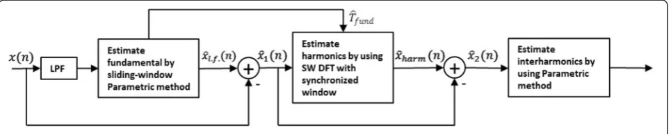
The Three-step Sliding-Window Hybrid method is a joint parametric-DFT scheme that was developed in three stages in which either the sliding-window (SW) ESPRIT, the SW Prony, or the SW DFT can be used alternatively to estimate (i) the fundamental and the interharmonic com-ponents in the 0 to 100 Hz band, (ii) the harmonics, and (iii) the interharmonics at frequency f> 100Hz of power system waveforms [29,30], reducing the typical problems that characterize the SW DFT and the SW parametric method (i.e., spectral leakage problems and high computa-tional efforts). Figure 3 shows the block diagram of the three-step method.
In more detail, in the first step, the SW parametric method (Prony or ESPRIT) is applied to the output of a low-pass band filter of 0 to 200 Hz, in order to estimate the power system's fundamental and the interharmonics in the frequency range from 0 to 100 Hz. Then, the fil-tered waveform is approximated with a linear combin-ation of exponentials according to either the (1) (SW ESPRIT) or (6) (SW Prony).
In the second step, the SW DFT is used to evaluate the harmonic components; in fact, there is also an estimation of the fundamental frequency among the outputs of the first step, so it is possible to set the duration of the DFT analysis window equal to an integer multiple of the funda-mental periodT^fund, greatly limiting the spectral leakage.
As shown in Figure 3, the waveform analyzed by the synchronized DFT is obtained by subtracting from the original signal x(n) the reconstructed waveform ^xl:f:ð Þn
that was obtained by the first step. The duration of the analysis window in this step can be set to 10 cycles
(12 cycles) of the fundamental periodT^fund, for 50-Hz
sys-tems (60-Hz syssys-tems), according to the IEC recommenda-tions, but if it is required, it also is possible to select a different number of cycles [29]. We note that the aforesaid synchronization of the DFT time window guarantees a very accurate estimation of the harmonic components with a reduced computational effort, and this is attribut-able to the significant limitation of the spectral leakage due only to the possible presence of interharmonics at fre-quenciesf> 100Hzinx1(n), which yields relatively low
er-rors [5,29].
The waveform x^harmð Þn in Figure 3 was obtained
sum-ming the estimated harmonics and using the results to compute the residualx2(n) by subtracting ^xharmð Þn from
x1(n). The waveformx2(n) is analyzed in the third step by
the same parametric method used in the beginning of the scheme.
Note that, in the first and third steps, the number of exponentials required in the model was considerably lower than the number needed in the application of SW ESPRIT or SW Prony to the full band signal. This posi-tive outcome resulted from the explanation of the de-composition of the waveform in different frequency ranges separately analyzed in the first and third steps. As a result, the Three-step SW method has a significantly lower computational burden than SW ESPRIT or SW Prony while still providing highly accurate results.
In order to improve the global performances of the Three-step SW method, each step could have a different duration of the analysis window, and then, the results could be processed and associated with a common time interval.
1.3.2 The sliding-window modified parametric method
The Sliding-Window Modified Parametric methods are based on a reduction of the unknown parameters in the signal model in the original parametric methods with ob-vious improvements in terms of computational efforts. In fact, starting from the consideration that the damping fac-tors and the frequencies of spectral components in power system applications are slightly variable versus time [25,39-43], the estimation of frequencies is conducted only a few times, and the damping factors are assumed to be constant along the entire signal to be analyzed [31,32].
Specifically, in [32], the frequencies of the spectral components were computed initially by the analysis of the first sliding window, thebasis window, and then, the values that were obtained were assumed to be constant with time, and they were imposed as known quantities in the successive sliding windows (no-basis windows). The damping factors were assumed to be null in the SW M-Prony and fixed to previously calculated values dur-ing the analysis of the ‘basis window’ in the SW M-ESPRIT [32].
We note that, to elude masking effects due to significant variation of the frequencies, it is expected that the estima-tion of the frequencies would be repeated periodically. If the deviation between the values obtained was greater than a fixed threshold, the frequencies are updated and the analysis restarts with these new values. We also note that a different choice is required for the damping factors in the Prony and ESPRIT methods. The damping factors, in fact, are able to take into account temporal variations of the amplitudes of the spectral components and to link two consecutive sliding windows smoothly.
When the duration of the windows is very short (one to two times the fundamental period), the damping factors have very low values, and their contribution is negligible. This is the case for the SW Prony, so for this method, the damping factors are set equal to zero. However, for the SW ESPRIT, the duration of the analysis window is signifi-cantly larger (four to five times the fundamental period), so in this case, the damping factors are assumed to be constant for the no-basis windows and equal to the damp-ing factors estimated for the basis window [32].
Figure 4 shows the block diagram of the Sliding-Window Modified Parametric methods.
In the first window (basis window for k=0), a trad-itional parametric algorithm (TPA) is used to estimate all of the unknown parameters ABWk ;fBWk ; ψBW
k ; αBWk
, which, then, are stored; in this window, the research for the optimal values for M and N1or N(respectively for
the ESPRIT-based and Prony-based method) is effected, updating them if the reconstruction error overcomes a prefixed threshold. The same algorithm is also used after kfwindows, where another basis window is generated in
order to avoid the masking effect. The choice of the valuekfis related to the particular nature of the analyzed
waveform. In theno-basis windows, a modified paramet-ric algorithm (MPA) is used only for the computation of the unknown amplitudesAk and initial phasesψkof the
spectral components, since the frequencies are equal to fBWk , and the damping factors are forced to be null or equal to αBW
k for the Prony and ESPRIT methods,
re-spectively. Specifically, the equations solved in the MPA when ESPRIT is used are as follows:
iÞ Rx¼VBWAV
When Prony is used, the equation system solved in MPA is as follows:
computational effort is reduced significantly compared to the classical Prony or ESPRIT approach [32].
1.4 Numerical applications
The basic and advanced parametric methods shown in Sections 1.2 and 1.3, respectively, were used to analyze the waveform distortion due to PVSs and WTSs, and the accuracy of their results and the computational bur-den of the methods were compared. Several numerical experiments were conducted, analyzing both synthetic and measured waveforms in many operating conditions of DG units, but for sake of brevity, only four case stud-ies are reported in this section, and all of them are re-ferred to the analysis of the current waveforms.
Specifically, the synthetic and measured currents of PVSs and WTSs were analyzed by using the following:
– the IEC standard method (IECM);
– the Sliding-Window ESPRIT method (SWEM); – the Sliding-Window Prony method (SWPM); – the Three-step Sliding-Window ESPRIT-DFT-ESPRIT
method (SWEDEM);
– the Three-step Sliding-Window Prony-DFT-Prony method (SWPDPM);
– the Sliding-Window Modified ESPRIT method (SWMEM);
– the Sliding-Window Modified Prony method (SWMPM).
The results of each case study were referred to the same duration of signal, and the IECM computational burden was considered as a reference for the other methods. It is important to emphasize that, for the IECM, since its frequency resolution was fixed at 5 Hz, the fundamental component was always detected in cor-respondence with 50 Hz, so the harmonic components are estimated also as multiples of 50 Hz.
All of the programs were conducted in MATLAB, and they were not optimized for computational speed be-cause we were interested only in obtaining a rough and relative quantification of the efficiency of the different methods. The MATLAB programs were developed and tested on a Windows PC with an Intel i7-3770 3.4 GHz and 16 GB of RAM.
1.4.1 Case study 1: test signal of a photovoltaic system
The synthetic 3-s waveform emulated a current at the PCC of a PVS that had a full-bridge, unipolar inverter. It was a sort of an ‘acid test,’since our aim was to observe the behavior of each of the methods in the analysis of a waveform with a very wide spectrum, i.e., exceeding a frequency of 20 kHz. Specifically, the waveform was as-sembled assuming a frequency modulation index mf
equal to 200 for the inverter PWM technique and the presence of all odd harmonics up to the 27th order for the low-frequency components. The fundamental com-ponent was fixed at 50.02 Hz, and it had an amplitude of 9 A. Also, a white noise with a standard deviation of 0.001 was added to the aforesaid components.
The sampling rate was 100 kHz in order to provide the most appropriate operating conditions for the para-metric methods that were used so that they could pro-vide estimates of the spectral components around the order 2mf, which are the most significant introduced by
the aforesaid type of PWM and whose amplitudes were fixed up to 12% of the fundamentala. For the parametric methods, the error threshold was fixed equal to 10−5, and for all of the methods, the window of analysis slides of 0.04 s was used. In the second steps of both SWPDPM and SWEDEM, the analysis window was fixed equal to 5 cycles of the fundamental period.
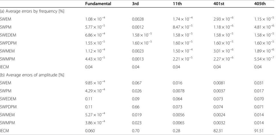
Table 1 shows the average percentage errors in the esti-mates of the frequencies and amplitudes of five spectral components, particularly interesting in the comparison of the methods that were used. Specifically, the components
that were examined were the fundamental and the har-monics of order 3rd, 11th, 401st, and 405th, with ampli-tudes equal to 1.6%, 6%, 12%, and 3% of the fundamental amplitude, respectively.
It was evident that SWEM, SWPM, SWMEM, and SWMPM always provided negligible percentage errors, with values almost of the same order of magnitude. As the first part of Table 1 shows, the percentage errors ob-tained using the SWEDEM and the SWPDEPM also were very low; however, the second part of Table 1 shows SWEDEM and SWPDEPM with higher errors for the amplitude than with the other basic and advanced parametric methods.
This behavior of the three-step methods in estimating the amplitudes of the fundamental and third harmonic was due to the presence of the low-pass band filter of 0 to 200 Hz, which introduces a little attenuation in the amplitude of the components in the frequency band of 0 to 100 Hz and slight distortions for the components near the filter cut-off frequency. However, it is important to emphasize that, for the other harmonic components (far from the filter cut-off frequency) both at low and high frequency, the errors in the amplitude were practic-ally negligible. Table 1 shows that the IECM errors were globally higher, both in terms of frequency and ampli-tude, and that, for the high-frequency components, the average percentage error in the estimation of amplitudes increased, reaching values greater than 90%.
This was due to the desynchronization between the dur-ation of the time window and the fundamental period,
Table 1 Case study 1: average percentage estimation errors
Fundamental 3rd 11th 401st 405th
(a) Average errors by frequency [%]
SWEM 1.08 × 10⁻⁴ 0.0028 1.74 × 10⁻⁴ 2.93 × 10⁻⁶ 1.15 × 10⁻⁵
SWPM 5.77 × 10⁻⁵ 0.0012 8.47 × 10⁻⁵ 1.18 × 10⁻⁶ 4.81 × 10⁻⁶
SWEDEM 6.86 × 10⁻⁴ 1.58 × 10⁻⁵ 1.58 × 10⁻⁵ 1.58 × 10⁻⁵ 1.58 × 10⁻⁵
SWPDPM 1.55 × 10⁻⁵ 1.60 × 10⁻⁵ 1.60 × 10⁻⁵ 1.60 × 10⁻⁵ 1.60 × 10⁻⁵
SWMEM 1.12 × 10⁻⁴ 0.0023 1.50 × 10⁻⁴ 3.01 × 10⁻⁶ 1.89 × 10⁻⁶
SWMPM 4.43 × 10⁻⁵ 0.0013 2.21 × 10⁻⁵ 2.27 × 10⁻⁶ 5.54 × 10⁻⁷
IECM 0.04 0.04 0.04 0.04 0.04
(b) Average errors of amplitude [%]
SWEM 9.85 × 10⁻⁴ 0.067 0.016 0.0081 0.031
SWPM 4.29 × 10⁻⁴ 0.026 0.0078 0.0037 0.017
SWEDEM 0.11 0.09 0.064 0.073 0.070
SWPDPM 0.11 0.66 0.073 0.074 0.071
SWMEM 5.27 × 10⁻⁴ 0.019 0.0056 0.0024 0.014
SWMPM 3.86 × 10⁻⁴ 0.023 0.0065 0.0032 0.014
IECM 0.060 0.70 0.28 82.31 91.51
which produces spectral leakage problems that increase as the harmonic order increases. Table 2 shows the computa-tional times obtained by using all of the methods to analyze the 3-s waveform per unit of computational time required by IECM. It is evident that the basic parametric methods require greater computational time in order to provide accurate results; however, the advanced paramet-ric methods reduced the computational effort significantly while simultaneously providing highly accurate results. Note that the SWEM (SWMEM) required less computa-tional effort than the SWPM (SWPEM); this was due to under-sampling the signal before analysis [44].
Tables 3 and 4 are provided to make it clearer what occurred in terms of the accuracy and computational ef-forts when the sampling rate in SWEM and SWMEM remained at 100 kHz. Table 3 shows that there was an irrelevant gain in the accuracy of the results compared to the values shown in Table 1.
However, the computational burdens of SWEM and SWMEM (Table 3) were considerably greater than those observed for the same methods in Table 2. This proves that the optimal sampling rate for each parametric method guarantees the best performance with respect to accuracy and computational time. It also proves that the accuracy of the results was not affected by exceeding the optimal sampling rate, but the computational effort in-creased significantly, especially at the very high-sampling rates.
Table 2 shows that the computational time of SWEDEM was greater than that of SWPDPM. This was because the presence of the filter in the first step resulted in some neg-ligible spectral components at low frequency that made it impossible to reduce the signal sampling rate in the first step of SWEDEM and maintain an acceptable accuracy.
It was interesting to observe that, in this case study, the advanced parametric methods required computational times that were, in the worst case (i.e., the SWEDEM and the SWMPM), an order of magnitude greater than that needed by the IECM. SWPDPM and SWMEM had com-putational times that were the same order of magnitude as that of the IECM, although these methods provided better
results than the method recommended by the IEC standards.
1.4.2 Case study 2: measurement of the current of the photovoltaic system
A 1-s current waveform measured at the PCC of a 10-kW, three-phase inverter without an isolation transformer, which, together with another twin-inverter, is included in a PVS. The sampling rate was 10 kHz, but in order to pro-vide better operating conditions for the detection of spec-tral components by the parametric methods that were used, a resampling to 20 kHz was used [44].
The error threshold for the parametric methods was fixed at 10−3, and the window of analysis slides of 0.04 s was used for all of the methods. In the second steps of the SWPDPM and the SWEDEM, the analysis window was fixed equal to 5 cycles of the fundamental period. Figure 5 shows the time trend of the measured current.
All of the methods that were used detected mainly low-frequency spectral components. In fact, in the fre-quency band from 5 to 10 kHz, the advanced methods that used the ESPRIT method and the DFT method de-tected the same components, but the values of ampli-tude were lower than the 0.05% of the fundamental, so they are not discussed here.
Table 5 shows the average values of frequency and amplitude of some spectral components detected by all of the methods that were used. Among the most signifi-cant spectral components, Table 5 reports the results re-lated to the fundamental, a harmonic at about 1,000 Hz, and an interharmonic at about 2,915 Hz. They are good representatives that provide a perception of the behav-iors of the methods that were used in the evaluation of the various types of spectral components.
First, as expected, it was evident that both harmonic and interharmonic components had low amplitudes and that each method was able to estimate them adequately, since the values that were obtained for both frequency and amplitude were in a narrow range.
The IECM provided an amplitude value of about 1 order of magnitude lower than the other methods only for the interharmonic detection, although the component was al-most a multiple of 5 Hz (the IECM frequency resolution). This phenomenon was compatible with the observation in the previous case study; in fact, it confirmed that spectral leakage increases at high frequencies.
Table 6 shows the computational time, per unit of the computational time required by IECM, obtained by ana-lyzing the current waveform by all of the methods. The advanced parametric methods always required less com-putational time than the basic parametric methods. In particular, all of the advanced parametric methods re-quired a computational time that was 2 orders of magni-tude less than those of SWEM and SWPM.
Table 2 Case study 1: computational time of all of the methods
Computational time [p.u.]
SWEM 45.56
SWPM 618.03
SWEDEM 12.86
SWPDPM 4.24
SWMEM 2.87
SWMPM 10.27
IECM 1
Also, in this case, the SWMEM was the method that came the closest to matching the performance of IECM with respect to computational time. Note that, for the analysis of the measured current, all of the advanced parametric methods required computational times that were only 1 order of magnitude greater than that re-quired by IECM.
1.4.3 Case study 3: test signal of wind turbine system
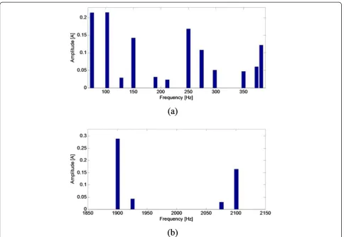
The synthetic 1-s waveform emulated a current at the PCC of a WTS that had a doubly fed induction generator. Also, this case study was a sort of‘acid test,’since our aim was to observe the behavior of each of the methods in the analysis of a waveform with a spectrum that exceeded a frequency of 2 kHz and that had embedded successive harmonic and interharmonic components.
The waveform was assembled assuming a frequency modulation index mf of 40, and the fundamental
fre-quency and amplitude were fixed at 50.02 Hz and 5.4 A, respectively. Figure 6 shows the low-frequency and the high-frequency spectrum of the test signal. White noise with a standard deviation of 0.001 was added to the sig-nal in order to make the waveform more realistic and to stress the performance of the spectral analysis methods that were used.
The sampling rate was 20 kHz. For the parametric methods, the error threshold was fixed at 5 × 10⁻⁸, and for all of the methods, the window of analysis slides was 0.04 s. In the second steps of both the SWPDPM and the SWEDEM, the analysis window was equal to 10 cy-cles of the fundamental period.
Table 7 shows the average percentage errors in the es-timates of the frequency and amplitude of the five
spectral components, which are particularly interesting for comparing the methods that were used. Specifically, the components that were examined were the funda-mental, the 5th, and the 38th order of harmonic and two interharmonics at 74.79 and 382.35 Hz.
In this case study, it was observed that the SWPM, in order to provide reasonably accurate results, requires a very high number of exponentials M, and as a result, it also requires a high value of N for the optimal window of analysis. This is due to the contemporaneous presence of noise interference and many small spectral compo-nents in the signal. In fact, since the Prony signal model does not include noise, Prony-based methods require an increasing number ofMin the presence of so many small spectral components and noise. Basically, the SWPM adds many spectral components to the real spectrum, since it also must individuate the noise spectrum to approach the analyzed waveform adequately.
However, it is easier for the SWEM to detect the spectrum, since noise is accounted for in its model.
However, as shown in Table 7, both the SWPM and the SWEM provide better results in terms of accuracy, with average percentage errors of the same order of magnitude. Obviously, noise interference also was a problem for the SWMPM, which produced less accurate results than the SWMEM; however, it performed well in detecting the spectral components, with errors of the same order of magnitude as the basic parametric methods (error of less than 0.021% for the estimation of frequency and less than 0.9% for the estimation of the amplitude). The sec-ond part of Table 7 shows that the SWPDPM and the SWEDEM had some difficulties in estimating the ampli-tudes of the components up to the fifth harmonic; as underlined in case study 1, this was due to the effect of the low-pass band filter. However, the first part of Table 7 shows that the average percentage errors for these methods were comparable to the best results obtained by the basic methods.
However, in the estimations of both the frequency and the amplitude, the IECM had the largest errors, espe-cially for the interharmonic components, which were de-tected with average percentage errors in the frequency
Table 3 Case study 1: average percentage estimation errors
Fundamental 3rd 11th 401st 405th
(a) Average errors of frequency [%]
SWEM 7.80 × 10⁻⁵ 0.0013 1.10 × 10⁻⁴ 1.53 × 10⁻⁶ 6.02 × 10⁻⁶
SWMEM 6.07 × 10⁻⁵ 7.39 × 10⁻⁴ 9.75 × 10⁻⁵ 3.22 × 10⁻⁶ 2.29 × 10⁻⁷
(b) Average errors of amplitude [%]
SWEM 5.30 × 10⁻⁴ 0.026 0.0092 0.0046 0.018
SWMEM 2.58 × 10⁻⁴ 0.029 0.0036 0.0034 0.014
Average percentage estimation errors of (a) frequency and (b) amplitude of spectral components detected by SWEM and SWMEM.
Table 4 Case study 1: computational time for the oversampled waveform
Computational time [p.u.]
SWEM 107.01
SWMEM 58.57
of 0.2% and 0.6% for the components near 74.79 and 382.35 Hz, respectively. For the same components, the average errors of amplitude were even worse, at 3% and 31%, respectively.
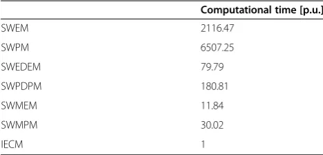
Table 8 shows the computational time required to analyze the test signal by all of the methods. Also in this case, the SWEM and the SWPM appear to be the slow-est methods, whereas the advanced parametric methods had computational times that were significantly less than those of SWEM and SWPM. In fact, in the best case, they were only 1 order of magnitude greater than the time required by IECM. In particular, once again,
SWMEM is the method that required a computational time that was the closest to that of IECM.
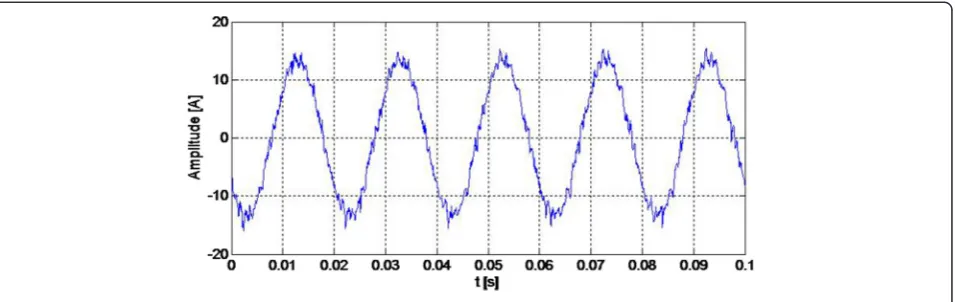
1.4.4 Case study 4: measured signal of wind turbine system
A 6-s current waveform measured during the soft start-ing of a fixed-speed wind turbine was analyzed. The ori-ginal sampling rate was 2,048 Hz, so a resampling at 10 kHz was conducted.
For the parametric methods, the error threshold was fixed equal to 10−7, and the window of analysis slides was 0.02 s for all of the methods. In the second steps of both the SWPDPM and the SWEDEM, the analysis window was fixed equal to 3 cycles of the fundamental period. Figure 7 shows the highly time-varying trend of this wave-form, which allowed us to test and compare methods also in the analysis of a non-stationary waveform.
As was predictable based on the theoretical consider-ations reported in Section 1.1, all of the methods identi-fied the 3rd, 5th, 7th, and 11th harmonics as significant components, in addition to the fundamental. The ampli-tudes of the aforesaid components were characterized initially by an increasing trend up to a maximum value, after which the descending phase began and continued until each component achieved its steady-state value.
Figure 5Case study 2: time trend of the analyzed current.
Table 5 Case study 2: average values
Fundamental Harmonic Interharmonic
(a) Average values of frequency [Hz]
SWEM 49.98 1001.38 2915.63
SWPM 49.97 1001.61 2914.50
SWEDEM 49.98 999.55 2911.02
SWPDPM 49.98 999.51 2912.03
SWMEM 49.98 1001.15 2912.28
SWMPM 49.97 1000.73 2912.00
IECM 50.00 1000.00 2915.00
(b) Average values of amplitude [A]
SWEM 13.44 0.18 0.15
SWPM 13.39 0.24 0.15
SWEDEM 13.38 0.23 0.14
SWPDPM 13.39 0.23 0.14
SWMEM 13.44 0.27 0.15
SWMPM 13.44 0.24 0.14
IECM 13.40 0.20 0.052
Average values of (a) frequency and (b) amplitude of the fundamental, a harmonic, and an interharmonic detected by SWEM, SWPM, SWEDEM, SWPDEPM, SWMEM, SWMPM, and IECM.
Table 6 Case study 2: computational time
Computational time [p.u.]
SWEM 9447.06
SWPM 5227.87
SWEDEM 21.59
SWPDPM 15.58
SWMEM 11.75
SWMPM 21.35
IECM 1
Figure 6Case study 3: spectrum of the WTS test signal. (a)Low-frequency spectrum;(b)high-frequency spectrum.
Table 7 Case study 3: average percentage errors
Fundamental 74.79 Hz 5th 382.35 Hz 38th
(a) Average errors of frequency [%]
SWEM 1.18 × 10⁻⁴ 0.0036 9.24 × 10⁻⁴ 0.0041 3.75 × 10⁻⁵
SWPM 7.84 × 10⁻⁵ 0.0013 4.35 × 10⁻⁴ 0.0015 2.39 × 10⁻⁵
SWEDEM 0.0056 0.0063 0.0042 0.0028 0.0042
SWPDPM 9.37 × 10⁻⁵ 0.0025 1.60 × 10⁻⁵ 0.0019 1.60 × 10⁻⁵
SWMEM 3.88 × 10⁻⁴ 0.0041 0.0028 0.021 5.18 × 10⁻⁵
SWMPM 0.0016 0.011 0.11 0.12 3.69 × 10⁻⁴
IECM 0.04 0.28 0.04 0.64 0.04
(b) Average errors of amplitude [%]
SWEM 0.0019 0.059 0.066 0.48 0.026
SWPM 0.0012 0.039 0.035 0.22 0.028
SWEDEM 0.19 2.80 2.01 0.43 0.25
SWPDPM 0.19 2.77 2.09 0.36 0.077
SWMEM 0.0014 0.027 0.20 0.89 0.011
SWMPM 0.0058 1.16 1.50 7.34 0.041
IECM 0.10 3.41 2.15 31.48 3.12
Table 9 reports the maximum peak values of ampli-tude for the fundamental, the fifth, and the seventh har-monics that were detected by the methods that were used.
The results presented in Table 9 provide evidence that the IECM had significant spectral leakage since the esti-mated values always were considerably lower than those obtained by the parametric methods. These lasts, in fact, estimate, for each component, values that differ slightly from each other.
Note that, as expected, the behaviors of the time trends of the frequencies were different; in fact, all of the parametric methods had spectral-component frequencies with negligible time variations.
Table 10 shows the computational time required by all of the methods to analyze the current's waveform. The results were similar to those in the previous case study. It is important to observe that the SWMEM required a computational time that was only double that of IECM.
2 Conclusions
In this paper, we analyzed some methods used to esti-mate waveform distortions caused by photovoltaic and wind turbine systems. An overview of the waveform
distortions caused by the most common configurations of PVSs and WTS schemes was also provided.
The theoretical aspects of the basic and advanced parametric methods proposed in literature were pre-sented, focusing on their high accuracy while, at the same time, emphasizing how the advanced parametric methods have the advantage of having computational times that are significantly less than those required by the basis parametric methods.
The basic parametric methods that were considered were the Sliding-Window ESPRIT method and the Sliding-Window Prony method. The advanced paramet-ric methods were the following:
the Three-step Sliding-Window ESPRIT-DFT-ESPRIT method;
the Three-step Sliding-Window Prony-DFT-Prony method;
the Sliding-Window Modified ESPRIT method; the Sliding-Window Modified Prony method.
These methods were used in the spectral analysis of synthetic and measured currents of PVSs and WTSs in order to compare them in terms of the accuracy of the results they produced and computational efforts for both stationary and non-stationary waveforms. The wave-forms were analyzed also by the IEC standard method, which we used as a reference for comparisons of compu-tational times.
The case studies that were considered highlighted the importance of an adequate sampling rate for the para-metric methods and the importance of the effect of noise on the detection of spectra by the Prony-based method when the signal components have very small amplitudes. In fact, in these cases, the ESPRIT-based methods can estimate the spectral components more easily, requiring a lower computational burden than the methods that use the Prony model.
Table 8 Case study 3: computational time
Computational time [p.u.]
SWEM 2116.47
SWPM 6507.25
SWEDEM 79.79
SWPDPM 180.81
SWMEM 11.84
SWMPM 30.02
IECM 1
Computational time, in p.u. of the computational time required by the IECM, of all of the methods.
All of the parametric methods were shown to have high levels of accuracy, exceeding that provided by the IECM, especially when the waveform spectrum was very wide. The IECM, in fact, failed in the detection of both interhar-monic components and high-frequency harinterhar-monics.
Conversely, the advanced parametric methods took less computational effort than the basic parametric methods, with computational times of the same order of magnitude or no more than 1 order or magnitude greater than that of the IECM. The aforesaid numerical experiments also demonstrated that the SWMEM gener-ally provided the best compromise between high-accuracy results and low computational effort.
It is important to note that, for very wide spectra, the three-step solution could inspire a new method for spec-tral analysis in which separating the waveform into low-and high-frequency components could result in the rapid and accurate detection of the spectral components of both the aforesaid bands by adapting the duration of the analysis window to the lowest frequency of each band.
3 Appendix A - IEC method
The standards IEC 61000-4-7 [23] and IEC 61000-4-30 [22] propose to use, for the spectral analysis of the non-stationary waveforms, the Sliding-Window Discrete Fou-rier Transform, which consists of applying the DFT to
consecutive windows that slide forward successively over time.
Ifx(n) is a waveform sampled data, it is possible to ob-tain the correspondingN-point DFT,X(k), as:
X kð Þ ¼X N−1
n¼0
x nð Þe−j2πNkn; k¼0;1;…;N−1 ð13Þ
The SW DFT, Xm(k), by definition, follows from the
(13), introducing, for the sampled waveform x(n) with length L, a window functionw(n), generally rectangular, with sizeN<L:
Xmð Þ ¼k XN−1
n¼0
x nð Þw nð −mÞe−j2πNkn; k¼0;1;…;N−1
ð14Þ
wheremis the starting time instant.
It is worth to observe that the aforesaid window func-tion is very important both in terms of analysis reso-lution and of spectral leakage. Specifically, it is important to choose adequately the time duration Tw of
the analysis window; in fact, for a sampling intervalTs, it
is Tw=NTs, and the frequency resolution of the
spectrum isf=1/Tw, so the selected valueNhas to be a
compromise to obtain a good resolution both in time and in frequency. According to the IEC standard, for a rectangular window, the compromise is a time duration Tw equal to 10 and 12 cycles of fundamental period,
re-spectively, for 50-Hz systems and 60-Hz systems [22,23]. Moreover, selecting a synchronized window with aTw
equal to an integer multiple of the waveform fundamen-tal period, it is also possible to avoid the spectral leakage phenomenon, which is the most significant problem of the DFT method, because it impacts negatively on the analysis results accuracy. In this regard, the time duration recommended by the IEC standards becomes generally in-adequate, especially in the presence of interharmonic components.
3.1 Endnote a
Note that, as shown in [44], if fs is the chosen sam-pling rate, the Prony's method is able to detect a max-imum component at a frequency of fs/4, whereas the ESPRIT method can estimate components up to fs/2. Then, the signal was under-sampled at 50 kHz before the application of SWEM and SWMEM.
Abbreviations
DER:distributed energy resources; DFIG: doubly fed induction generator; DFT: Discrete Fourier Transform; DG: dispersed generation; IEC: International Electrotechnical Committee; IECM: IEC standard method; MPPT: maximum power point tracking; PCC: point of common coupling; PQ: power quality; PVS: photovoltaic system; PWM: pulse-width modulation; SCIG: squirrel-cage induction generator; SG: smart grid; SW: sliding-window; ESPRIT: estimation of signal parameters by rotational invariance technique; SWEDEM: Three-step Table 9 Case study 4: estimated peak values
Maximum peak value [A]
Fundamental 5th 7th
SWEM 866.92 139.96 66.97
SWPM 857.84 139.79 64.56
SWEDEM 867.06 139.31 64.14
SWPDPM 867.68 139.26 63.90
SWMEM 864.24 143.03 70.99
SWMPM 867.52 140.25 67.19
IECM 814.20 133.40 58.50
Peak values of the fundamental, 5th, and 7th harmonics detected by SWEM, SWPM, SWEDEM, SWPDEPM, SWMEM, SWMPM, and IECM.
Table 10 Case study 4: computational time
Computational time [p.u.]
SWEM 145.44
SWPM 367.38
SWEDEM 25.34
SWPDPM 57.26
SWMEM 2.34
SWMPM 4.29
IECM 1
Sliding-Window ESPRIT-DFT-ESPRIT method; SWEM: Sliding-Window ESPRIT method; SWMEM: Sliding-Window Modified ESPRIT method;
SWMPM: Sliding-Window Modified Prony method; SWPDPM: Three-step Sliding-Window Prony-DFT-Prony method; SWPM: Sliding-Window Prony method; THDi: current total harmonic distortion; WTS: wind turbine system.
Competing interests
The author declares that she has no competing interests.
Received: 30 October 2014 Accepted: 6 January 2015
References
1. E Santacana, G Rackliffe, X Feng, Getting smart. IEEE Power Energ Mag 8(2), 41–48 (2010)
2. H Farhangi, The path of the smart grid. IEEE Power Energ Mag 8(1), 18–28 (2010)
3. RH Lasseter, Smart distribution: coupled microgrids. Proc IEEE 99(6), 1074–1082 (2011)
4. A Vojdani, Smart integration. IEEE Power Energ. Mag.6(6), 71–79 (2008). November-December
5. P Caramia, G Carpinelli, P Verde,Power quality indices in liberalized markets (Wiley-IEEE Press, New Jersey, 2009)
6. F Blaaiberg, Z Chen, SB Kjaer, Power electronics as efficient interface in dispersed power generation systems. IEEE Trans Power Electron 19(5), 1184–1194 (2004)
7. R Angelino, A Bracale, G Carpinelli, M Mangoni, D Proto, Dispersed generation units providing system ancillary services in distribution networks by a centralized control. IET Renew Power Gener5(4), 311–321 (2011) 8. CIGRE WG 37–23: Impact of increasing contribution of dispersed generation
on the power system (1999)
9. F Gronwald, Frequency versus time domain immunity testing of smart grid components. Adv Radio Sci12, 149–153 (2014)
10. RC Variath, MAE Andersen, ON Nielsen, A Hyldgard, A review of module inverter topologies suitable for photovoltaic systems. in IPEC, 2010 Conference Proc., Singapore, 27–29 October 2010
11. SA Papathanassiou, MP Papadopoulos, Harmonic analysis in a power system with wind generation. IEEE Trans Power Delivery21(4), 2006–2016 (2006) 12. ST Tentzerakis, SA Papathanassiou, An investigation of the harmonic
emissions of wind turbines. IEEE Trans Energy Convers22(1), 150–158 (2007) 13. AE Feijoo, J Cidras, Modeling of wind farms in the load flow analysis. IEEE
Transactions on Power Systems15(1), 110–115 (2000)
14. JI Herrera, TW Reddoch, JS Lawler, Harmonics generated by two variable speed wind generating systems. IEEE Trans Energy Convers
3, 267–273 (1988)
15. MHJ Bollen, K Yang, Harmonic aspects of wind power integration. J Modern Power Syst Clean Energy1(1), 14–21 (2013)
16. IEC 61400–21: Wind turbine generator systems, part 21: measurement and assessment of power quality characteristics of grid connected wind turbines (2001)
17. L Alfieri, A Bracale, P Caramia, G Carpinelli, Advanced methods for the assessment of time varying waveform distortions caused by wind turbine systems. Part I: theoretical aspects. in 13th Int. Conf. on Environment and Electrical Engineering, EEEIC 2013, Poland, November 2013
18. SK Rönnberg,MH Bollen(EOA Larsson, Emission from small scale PV-installations on the low voltage grid. Renewable Energy and Power Quality Journal, 2014)
19. D Gallo, R Langella, A Testa, JC Hernandez, I Papic, B Blazic, J Meyer, Case studies on large PV plants: harmonic distortion, unbalance and their effects. in Power and Energy Society General Meeting (PES), IEEE , 21–25 July 2013 20. SK Ronnberg, K Yang, MHJ Bollen, AG de Castro, Waveform distortion - a
comparison of photovoltaic and wind power. in 16th Int. Con. on Harmonics and Quality of Power, Bucharest, Romania, 25–28 May 2014 21. A Andreotti, A Bracale, P Caramia, G Carpinelli, Adaptive Prony method for
the calculation of power quality indices in the presence of non-stationary disturbance waveforms. IEEE Trans Power Delivery24(2), 874–883 (2009) 22. IEC standard 61000-4-30: Testing and measurement techniques–power
quality measurement methods (2008)
23. IEC standard 61000-4-7: General guide on harmonics and interharmonics measurements, for power supply systems and equipment connected thereto (2009)
24. P Ribeiro,Time-Varying Waveform Distortions in Power Systems(John Wiley & Sons, New York, 2009)
25. GW Chang, C-I Chen, Measurement techniques for stationary and time-varying harmonics. in IEEE Power & Energy Society General Meeting 2010, PES 2010, Minneapolis, USA, July 2010
26. PM Silveira, C Duque, T Baldwin, PF Ribeiro, Sliding window recursive DFT with dyadic downsampling—a new strategy for time-varying power harmonic decomposition. in IEEE Power & Energy Society General Meeting, Canada, 2009
27. A Bracale, P Caramia, G Carpinelli, Adaptive Prony method for waveform distortion detection in power systems. Int J Electrical Power Energ Systems 29(5), 371–379 (2007)
28. I Gu, MHJ Bollen, Estimating interharmonics by using sliding-window ESPRIT. IEEE Trans on Pow Del23(1), 13–23 (2008)
29. A Bracale, G Carpinelli, IYH Gu, MHJ Bollen, A new joint sliding-window ESPRIT and DFT scheme for waveform distortion assessment in power systems. Electr Power Syst Res88, 112–120 (2012)
30. L Alfieri, A Bracale, P Caramia, G Carpinelli, Waveform distortion assessment in power systems with a new three-step sliding-window method. in 12th Int. Conf. EEEIC, EEEIC 2013, Wroclaw, Poland, 5–8 May 2013
31. J Zygarlicki, M Zygarlicka, J Mroczka, KJ Latawiec, A Reduced, Prony's method in power-quality analysis—parameters selection. IEEE Trans Power Delivery25(2), 979–986 (2010)
32. L Alfieri, G Carpinelli, A Bracale, New ESPRIT-based method for an efficient assessment of waveform distortions in power systems. Electr Power Syst Res 122, 130-139 (2015)
33. N Mohan,WP Robbins, TM Undeland, Power Electronics: Converters, Applications, and Design(Wiley, New York, 1995)
34. H Li, Z Chen, Overview of different wind generator systems and their comparisons. IET Ren. Pow. Gen. 2(2), 123–138
35. E Muljadi, N Samaan, V Gevorgian, Jun Li, S Pasupulati, Short circuit current contribution for different wind turbine generator types. in IEEE PES General Meeting, Minneapolis, United States, 25–29 July 2010
36. GL Xie, BH Zhang, Y Li, CX Mao, Harmonic propagation and interaction evaluation between small-scale wind farms and nonlinear loads. Energies 6, 3297–3322 (2013)
37. R Roy, T Kailath, ESPRIT - estimation of signal parameters via rotational invariance techniques. IEEE Trans. on Ac., Sp., and Sig. Proc. 37(7), 984–995 (1989)
38. A Bracale, P Caramia, G Carpinelli, Optimal evaluation of waveform distortion indices with Prony and RootMusic methods. Int J of Pow & En Syst27(4), 360–370 (2007)
39. T Lobos, Z Leonowicz, J Rezmer, P Schegner, High-resolution spectrum estimation methods for signal analysis in power systems. IEEE Trans Instrum Meas55(1), 219–225 (2006)
40. A Bracale, G Carpinelli, Z Leonowicz, T Lobos, J Rezmer, Measurement of IEC groups and subgroups using advanced spectrum estimation methods. IEEE Trans on Instr Meas57(4), 672–681 (2008)
41. A Bracale, P Caramia, G Carpinelli, A Rapuano, A new, sliding-window prony and DFT scheme for the calculation of power-quality indices in the presence of non-stationary waveforms. Int. J. of Emerging Electric Power Systems. 13(5), 6 (December 2012)
42. C-I Chen, GW Chang, An efficient Prony-based solution procedure for tracking of power system voltage variations. IEEE Trans Ind Electron 60(7), 2681–2688 (2013)
43. A Testa, MF Akram, R Burch, G Carpinelli, G Chang, V Dinavahi et al., Interharmonics: theory and modeling. IEEE Trans Power Del 22(4), 2335–2348 (2007)