Rate distortion optimized multi view streaming in wireless environment using network coding

(1)

R E S E A R C H

Open Access

Rate-distortion-optimized multi-view

streaming in wireless environment using

network coding

Claudio Greco

1

, Irina D. Nemoianu

2

, Marco Cagnazzo

3*

and Béatrice Pesquet-Popescu

3

Abstract

Multi-view video streaming is an emerging video paradigm that enables new interactive services, such as 3D video, free viewpoint television, and immersive teleconferencing. Because of the high bandwidth cost they come with, multi-view streaming applications can greatly benefit from the use of network coding, in particular in transmission scenarios such as wireless network, where the channels have limited capacity and are affected by losses. In this paper, we address the topic of cooperative streaming of multi-view video content, wherein users who recently acquired the content can contribute parts of it to their neighbors by providing linear combinations of the video packets. We propose a novel method for selection and network encoding of the transmitted frames based on the users’

preferences for the different views and the rate-distortion properties of the stream. Using network coding enables the users to retrieve the content in a faster and more reliable manner and without the need for coordination among the senders. Our experimental results prove that our preference-based approach provides a high-quality decoding even when the uplink capacity of each node is only a small fraction of the rate of the stream.

Keywords: Multi-view video coding, Network coding, Video streaming

1 Introduction

In recent years, the advances in video acquisition, com-pression, transmission, and rendering have made possi-ble the development of technologies that can enhance the viewers’ experience by including the third dimen-sion. While traditional 2D video offers the viewer only a passive view of the scene, a more realistic experience can be obtained through applications such as 3D video or free viewpoint selection. 3D cinema productions have already generated big revenues, but other applications such as 3DTV and Free Viewpoint TV (FTV) [1, 2] are also becoming more desirable due to the increased afford-ability of 3D displays for home use.

Multi-view video(MVV) is one of the key elements of these applications; it consists in the simultaneous repre-sentation of a scene captured by N cameras placed in different spatial positions, called points of view.

*Correspondence: [email protected]

3LTCI, CNRS, Télécom ParisTech, Université Paris-Saclay, 75013, Paris, France Full list of author information is available at the end of the article

By using more than two cameras during video acquisi-tion, adjacent views act like local stereo pairs to guarantee stereoscopy to the viewer. This can be used to synthe-size virtual views different from the acquired ones. This functionality is used in FTV where the user interactively controls the viewpoint in the scene. On the other hand, since 3D video could not be deployed if the quality per-ceived by the user does not exceed the existing 2D quality standards, the bandwidth for storage and transmission of the multiple views is accordingly increased.

A first solution for multi-view video transmission, known assimulcast[3], is to compress and send each view independently [4]. While simple to implement and back-ward compatible with the existing infrastructures, this technique does not take into account the redundancy due to the similarities among the views that can be used to fur-ther compress the data. On the ofur-ther hand, it allows for easier switching between views, as the lack of inter-view prediction makes the views independently decodable.

The multi-view video coding (MVC) extension of the H.264/MPEG-4 AVC standard [5] exploits inter-view dependency in a simple, yet effective ways; images from

(2)

other views (but at the same time instant) can be used as references for the current frame prediction (inter-view prediction). This is the only major change introduced in the MVC extension of H.264. The MVC extension of HEVC, referred to as MV-HEVC, is based on very simi-lar principles [6]. With MVC, two main coding schemes are particularly worth mentioning: view progressive and fully hierarchical. In the view progressive architecture, the first view, called the base view, is encoded inde-pendently from the others. In any other view, for each GOP, there is one frame, the V-frame, that is predicted using only inter-view prediction from the corresponding I-frame in the base view. For all other frames, only tem-poral prediction is used. In the second architecture, both hierarchical temporal prediction and inter-view predic-tion are performed for all P/B-frames of all views except for the the base view. These tools allow a rate reduc-tion, for the same subjective quality, estimated around 50 % with respect to the case of independent view coding (simulcast) [5].

Even though recently a relevant part of the attention of the research in 3D has been attracted by depth-based formats [7] (which allow virtual viewpoint synthesis), the interest in MVV coding is still very high, as witnessed by the activity of the ad hoc group on free viewpoint TV and super-multi-view video (i.e., video with more than 30 views, and holoscopic video) [8–10]. The quality of synthesized view generated with depth data is still ques-tionable, at such a point that it is still not completely clear whether depth-based format has a clear advantage over MVV or super-MVV, above all when subjective quality is considered [11]. In summary, super-MVV seems still being a serious candidate for FTV and 3D video services [12].

Multi-view streaming becomes an even more challeng-ing task in the context of mobile networkchalleng-ing, where the high bitrate issue of multi-view adds on top of the existing problems of mobile networking. Even though streaming applications are nowadays commonplace, and the tech-nology involved has greatly advanced in the past few years [13, 14], in a wireless network, it is difficult to meet the inherent requirement of continuous delivery necessary for an uninterrupted presentation of the content, as the nodes move freely and independently in all directions—thus, the channel conditions of the links and the link themselves are unreliable and erratic—and individual nodes may connect and disconnect asynchronously [15].

Also, in the context of a streaming application, it would be desirable to have the quality of the received media degrade gracefully as the network environment and resources change and to tolerate losses to some extent. Even though techniques to provide graceful degradation and loss immunity exist, these usually require an increase in the bitrate of the stream, a condition that could be

difficult to satisfy in a wireless network, where the nodes’ uplink capacity is typically quite limited.

One positive aspect of wireless networks w.r.t. video streaming is the inherently broadcast nature of the medium. This makes more straightforward for a sender the task of multicasting the content to several receiver but also allows a single receiver to collect video packet from several servers.

Recently, good results have been achieved, in the context of mobile video streaming, by exploiting the broadcast nature of the medium through the construction of video packet delivery overlays [16, 17]. These logical networks, built on top of the actual wireless network through the cooperation of nodes, allow to provide a streaming service with good video quality and graceful degradation.

However, these techniques were designed for single-view streams and relied on the use of multiple description coding (MDC) [18], a joint source-channel coding tech-nique that does not lend itself well to be conjugated with multi-view, due to its additional bitrate cost, a cost already considerable for multi-view streams.

In this article, we propose to use network coding for the robust delivery of MVV and super-MVV over an unreli-able network such as a wireless network. In order to do so, we design arate-distortion-optimized(RDO) scheduling algorithm that, at each sending opportunity, selects which video packet has to be added to the coding window, in such a way as to minimize the expected video distortion measured at the receiver. This optimization will be per-formed by taking into account the preferences of the users in terms of required views, an approach already success-fully exploited for video caching of single-view streams in mobile environment [19]. Being the wireless medium inherently broadcast, we exploit the fact that each receiver could be exposed to multiple senders. We thus ensure that senders transmit innovative packets (i.e., packets with novel information with respect to those already sent) even though they do not coordinate their actions.

The particularity of the coding structures of the multi-view representation reflects in a non-trivial impact of each coded frame on the overall quality of the recon-structed multi-view content. If this impact is properly captured, it can be used to design an intelligent transmis-sion scheme that allocates the limited channel capacities in a rate-distortion-optimized order (scheduling). In order to effectively disseminate the content to the end users, an analogous scheme can be devised to schedule the frames for transmission [20].

(3)

needed to reconstruct the original packets, are typically sent along the combinations as headers [22–25], unless more advanced reconstruction schemes are implemented at the receiver side [26, 27]. Used as an alternative to tra-ditional routing, NC has proved beneficial to real-time streaming applications, both in terms of maximization of the throughput and in terms of reduction of the effects of losses [28–33].

In a NC-based transmission system, rather than send-ing the data packets, the users send mixed packets. The advantage of this technique is that even though the users act independently from each other, with high probability, each of them will contribute innovative information to the transmission [20, 34]. In the most common implementa-tion of network coding, referred to as practical network coding (PNC) [25], the content is divided into groups of packets known asgenerations, and only packets belonging to the same generation can be mixed together. In our sys-tem, each packet contains only one encoded frame, and we only mix frames belonging to the same GOP. The set of packets actually used to generate a mixture is referred to ascoding window.

One technique based on the network coding princi-ples has been proposed by Wang et al. [35] for peer-to-peer video-on-demand applications. More recently, Kao et al. [36] proposed a general framework able to pro-vide an interactive streaming service, i.e., allowing random access operations to the users. However, neither of these techniques addresses the multi-view case, nor takes into account the rate-distortion properties of the stream, nor the users’ preferences.

Other existing works have tackled the subject of dis-tributed video services, achieving similar properties, by proposing to use rateless codes—conceptually similar to network coding—for video delivery [37, 38]. How-ever, even though these techniques have been proposed for video delivery, only the delay requirements of video streaming have been exploited, while our method is tai-lored for multi-view video content and in particular it uses the prediction structure of the encoded sequence in its optimization algorithm. It should be noted that in our method, a proper RDO-based scheduling is performed in order to provide the users with the best possible video quality given the limited channel capacity allocated to each node.

The rest of this article is organized as follows. In Section 2, we review some recent works closely related to our problem. Then, in Section 3, we present the sys-tem model, detailing and motivating our assumptions. In Section 4, we describe the selection method used to decide which frames will be included in the coding win-dow of the transmitting nodes. In Section 5, we present the experimental validation of the proposed technique and analyze the results. Finally, in Section 6, we draw

our conclusions and point out some directions for future work.

2 Related work

Unlike previous works on multi-view streaming rather than focusing on the source encoding of the content, and rather than considering each client as an independent agent, we study how the distribution of the stream can take advantage of an a priori knowledge about the dif-ferent clients and, in particular, the fact that they share common preferences—in this case, in terms of preferred view.

Examples of work in the context of multi-view stream-ing that take user preferences into account include the source rate allocation technique proposed in [39] and the joint source-channel coding scheme introduced in [40].

While these works consider similar applications as ours, we address here a substantially different problem, in which the multi-view video has been already encoded, and we must decide, at each sending opportunity, about which parts of the content have to be included in the cod-ing window for transmission. We also consider the case when the preference estimation used to decide the packet scheduling does not perfectly correspond to the actual user preferences.

In our work, we also rely on a network coding scheme that allows for the prioritization of certain packets with respect to others. Several works exist that make use of similar schemes, in which the video stream is divided into layers of priority and unequal error protection is given to the different layers using PNC.

For instance, in [29], a receiver-driven network coding strategy is proposed, where the receiving peers request packets from classes with varying importance. Packet classes are constructed based on the unequal contribu-tion of the various video packets to the overall quality of the presentation or in scalable video streams. Prioritized transmission is achieved by varying the number of packets from each class that are used in network coding opera-tions. The coding operations are driven by the children nodes that determine the optimal amount of coding allo-cated to each importance class of the data to which they subscribe.

(4)

be decoded, most likely the reference view from which it depends has been already received.

This work is related to ours both for its use of network coding and its application to multi-view content. How-ever, there are notable differences both in the model of the service provided to the user and, as a consequence, to the utility function that is maximized.

In the scenario envisioned in this work, users request viewpoints that are, in general, synthesized from cam-era views either by coinciding with one them or by using depth-image-based rendering on a couple of camera views bracketing the synthetic viewpoint. The distortion to minimize depends on the spatial distance between the synthetic view and each of the camera views used to reconstruct it. Priority, in the sense of a higher redun-dancy to insure reception in the face of losses, is defined based on the utility of camera view subsets in reconstruct-ing the synthetic views requested by the users.

In our work, on the other hand, the users are only inter-ested in camera views, i.e., no view synthesis is used. This implies that, while in the abovementioned work, there are different combinations of received camera views that can satisfy the view request of a user, with different levels of distortion depending on their distance; in our scheme, only the exact camera view the user is interested in can increase its quality of experience.

Furthermore, in our scheme, priority is not intended in the sense of loss protection but rather the arrival order. In our scheme, the different treatment of layers is not intended to differentiate the likelihood of their reception but rather the delay experienced by the user before they can start displaying it. For this reason, while the network coding scheme used in [41] varies the number of pack-ets from each layer in the coding window, in our scheme, all packets from lower layers are introduced in the coding window before any packet of a higher layer is introduced.

Notice that this work only considers the case of aligned and equally spaced cameras, so that correlation between views decreases with their distance. In a more recent work [42], the same authors extend this model to opti-mize other settings, but this work does not address the communication aspects.

Another relevant approach to video transmission from multiple senders is proposed in [43], wherein the authors jointly tackled the problem of defining an optimal sched-ule and an optimal network coding strategy using a priori-tizing network coding scheme. Unlike ours, this work only considers the case of single-view content, therefore there are no preferences to be taken into account, and the opti-mal schedule is unique. Furthermore, in order to find an optimal solution, this technique requires some degree of coordination among the senders, whereas, we assume that coordination is not feasible and relies on randomization in order to circumvent this limitation.

3 System model

In order to optimize the rate-distortion performance of the transmitted content, we select the frames to be included in the coding window based on their popularity among the users. Before explaining in detail our proposed technique, in this section, we list and justify some assump-tions about the system that will be used in the design of the technique.

• From the point of view of the network, we assume that the users are connected in a (generally partial) mesh network in which each node can potentially receive from multiple servers. This reflects the case of wireless networks and in particular ad hoc networks. Furthermore, we assume that the connectivity among the users can be modeled with a set of independent channels, each of them having a given capacityC, expressed as a fraction of the encoded video bitrate. WhenC=100 %, each node is able to transmit all the packets of a GOP in the time allocated to a GOP. Still, these packets may be lost on the channels. We consider two models for these channels: a simple packet erasure channel (PEC) with loss rateε, and a Gilbert-Elliot erasure channel (GE), characterized by loss rates in good and bad state (εGandεB) and by transition probabilities (pGBandpBG). Notice that each channel does not necessarily provide sufficient capacity for transferring the whole multi-view stream. Our study will focus on the video quality achieved by a generic receiverR exposed to M senders or sources S1,. . .,SM. This scenario is represented in Fig. 1.

• From the point of view of the content, we assume that the stream is encoded using H.264/MVC [5] or a similar inter-view prediction scheme, such as MV-HEVC [6]. In our experiments, the stream is encoded using the prediction structure depicted in Fig. 2, withM=5views andN=8 pictures per view in a GOP. This structure is a compromise between view progressive and fully hierarchical MVC that uses inter-view prediction in order to achieve a better coding efficiency but is not fully hierarchical in order to reduce the dependencies among the frames, thus reducing the propagation of the effects of losses. However, it should be noted that our study can easily be extended to other coding techniques and

prediction structures of multi-view content.

(5)

Fig. 1Simulated scenario for each receiver.I(v,k)andI(v,k)are, respectively, the original and reconstructed version of framekof viewv.

Sm,m=1,. . .,Mare the senders (or sources), NCmthe network coding modules, Cmthe capacity of the channels, RX is the receiverR’s buffer

learned and spread over the network with approaches similar to those shown in [17].

• We assume that the preference distribution does not change too fast over time, that is, we assume that it can be considered valid for at least the duration of a GOP, defined as an independently decodable set of N×Wframes, as depicted in Fig. 2. This implies that our system is able to work even when users’

preferences change as frequently as once per GOP, which typically lasts less than 1 s. Any change in preferences during a GOP will be taken into account at the next GOP.

An example of the complete system is shown in Fig. 3. The video server S sends the encoded video packets together with side information about RD characteristics of the sequence. Nodes 1 to 9 relay the video using the proposed system.

We focus on a given node receiving the video sequence fromMsources (or senders), performing network coding and relaying the video to downlink nodes. For example, node 6 sees M = 4 sources, i.e., nodes 1 to 4. Node 8 seesM = 2 sources, i.e., nodes 5 and 6. We propose an algorithm to decide the order of inclusion of frames in the coding window. We assume (for simplicity) that nodes do

(6)

Fig. 3Example of network for the proposed method. Nodesis the encoder. Node 6 seesM=4 sources (or senders). Node 8 seesM=2 sources

not compete for capacity but the available capacity may be less than the video coding bitrate. We model each chan-nel’s capacity as a percentage of the encoded video bitrate, and that each node has view preferences according to a given probability distribution.

4 Proposed method

In this section, we describe our proposed method of net-work encoding for a wireless streaming of multi-view video content based on the users’ preferences.

As we mentioned in Section 1, most practical imple-mentations of NC are achieved by segmenting the data flow into generations and combining only packets belonging to the same generation. Packets are made of the same length by padding. All packets in a gen-eration are jointly decoded as soon as enough linearly independent combinations have been received, by means of linear system solving. Since the coefficients are taken from a finite field, perfect reconstruction is assured.

It has been proposed [29] to apply NC to video content delivery, dividing the video stream into layers of priority and providing unequal error protection for the different layers via PNC. Layered coding requires that all users receive at least the base layer, hence all received packets must be stored in a buffer until a sufficient number of independent combinations are received, which introduces a decoding delay that may be undesirable in real-time streaming applications.

There exist several techniques aimed to reduce the decoding delay, proposed by both the NC and the video coding communities. In our technique, we use an imple-mentation of random linear network coding referred to asexpanding window network coding (EWNC) [28, 32]. The key idea of EWNC is to increase the size of the coding window (i.e., the set of packets in the genera-tion that may appear in combinagenera-tion vectors) for each new packet. Using Gaussian elimination at the receiver side, this method provides instant decodability of packets.

Thanks to this property, EWNC is preferable over PNC in streaming applications. Even though PNC could achieve almost instant decodability using a small generation size, this would be ineffective in a wireless network, where a receiver could be surrounded by a large number of senders, and if the size of the generation is smaller than the number of senders, some combinations will necessarily be linearly dependent. On the other hand, EWNC auto-matically adapts the coding window size allowing early decodability, and innovation (i.e., linear independence) can be achieved if the senders include the packets in the coding window in a different order. However, these orders should take into account the RD properties of the video stream. In our previous work, we already success-fully applied EWNC principles to multi-view streaming in the context of wireless networking [44], but we did not take into account the preferences of the users in terms of displayed view.

As mentioned in Section 1, in other works, user pref-erences were used to optimize the rate allocation in the encoding process. Here, we show how they can be used to decide which parts of the content have to be included in the coding window in order to optimize the rate-distortion properties of the transmitted stream.

We model the distribution of users’ preferences with a probability vectorp, such thatpvis the probability that a

member of the group chooses to watch viewv∈ {1,. . .N} for the current GOP.

In our case, the transmitted packets will contain lin-ear combinations of frames belonging to the same GOP. In order to select the order in which the frames will be included in the coding window, which we denote byW, we proceed as follows. For each GOP, all the frames of the current GOP are stored in a bi-dimensional frame buffer

(7)

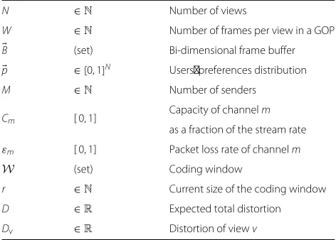
Table 1Summary of the notation used in this article

N ∈N Number of views

W ∈N Number of frames per view in a GOP

B (set) Bi-dimensional frame buffer

p ∈[0, 1]N Users’ preferences distribution

M ∈N Number of senders

Cm [ 0, 1]

Capacity of channelm

as a fraction of the stream rate

εm [ 0, 1] Packet loss rate of channelm

W (set) Coding window

r ∈N Current size of the coding window

D ∈R Expected total distortion

Dv ∈R Distortion of viewv

the GOPNW, while the current size of the coding window will be denotedr≤NW.

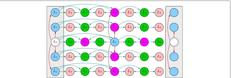
The organization of the bi-dimensional buffer cor-responding to the prediction structure described in Section 3 and depicted in Fig. 2 is shown in Fig. 4. Notice that the views are re-arranged to reflect the coding order, so the central view in Fig. 2 corresponds to view 1 in Fig. 4, as the other views are predicted upon it.

The scheduling Algorithm 1 aims to minimize the expected total distortion given a numberr≤NWof frames to be included in the coding window W. It works in an iterative fashion, starting with an empty coding window (W ← ∅) and adding at each iteration the most suit-able frame toW, given the frames already included at the previous iteration. More precisely, letDv(W) be a

func-tion that computed the distorfunc-tion of the viewvwhen the frames selected inW are available. Note that, due to the inter-view prediction, the functions Dv(·)depend on all

Fig. 4BufferBforN=5 views andW=8 frames for the structure in Fig. 2. In each view, frames are ordered by prediction level, then by descending impact on the total distortion of the view

the selected frames. For a generic user, the expected total distortionDis expressed as:

D(W)=

N

v=1

pvDv(W)= pD(W), (1)

Algorithm 1Algorithm used by the nodes to include the frames in the coding window

1: procedureSCHEDULEFRAMES

2: G←N×W; Size of the generation.

3: for allMV-GOPsdo

4: W← ∅; Coding window.

where vector D(W) is such that its vth component is Dv(W). The optimization problem can therefore be stated

as:

Algorithm 1 provides a heuristic way to computeW∗(r) for all r ∈ {1, 2,. . .,NW} with the additional con-straint that for all r, W∗(r − 1) is a subset of W∗(r), that is, W∗(r) is built by adding a frame to W∗(r − 1). In general, the optimal solution to this problem is unique. This means that all the senders would always compute exactly the same scheduling order. As a conse-quence, the “randomness” of NC would be lost; all the senders always transmit dependent combinations. Even if a node receives packets from M > 1 senders, they will be identical, defeating the purpose of using NC. In order to take advantage of the benefits of NC in terms of loss resiliency, we need to generate a variety of sched-ules, possibly slightly sub-optimal, but with acceptable performances.

(8)

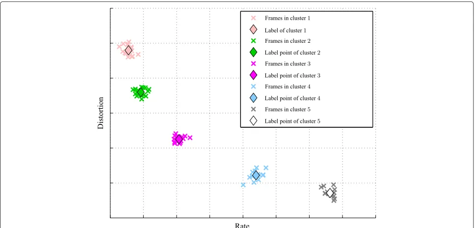
preferences into account. An illustration of the cluster-ing is given in Fig. 5. We observe that frame or packet classification based on RD properties has been used in the literature, for example, by Chakareski and Frossard [45]. However, beside the differences in computing or estimat-ing rate and distortion, we use classification in a totally different way, i.e., for achieving a scheduling diversity to be used in network coding. This concept is original in scientific literature.

The labels are decided only once at the encoder side, where rate and distortion are known with negligible com-putational overhead and where a best estimation of the receiver’s preferences is more likely to be available. Since the encoder knows the rate and distortion characteristics of the frames, it can send them to the users with a very little overhead, since this information amounts to a few bytes per frame.

Let us now describe in detail how Algorithm 1 works in an intermediate node. For all MV-GOPs, the node com-putes the coding window, starting with an empty set and adding at each sending opportunity a new frame. For a new value ofr, first, we compute the set of eligible frames F. It is made up of those whose references for predic-tion, if any, are already in the coding window. For example, whenW = ∅, only the intra-frame of the GOP is eligible. Therefore for all the nodes, when r = 1, W only con-tains the intra-frame. In general however,F contains all the frames that are decodable using only the frame inW and that are not inW (Algorithm 1, line 6), that is, for the second iteration, all the frames of levelL1with respect

to Fig. 4. For each frame inF, the algorithm computes the coding cost function Jf obtained by addingf to W.

Without clustering, generally speaking, a unique frame f would minimize Jf, making it impossible to produce

different scheduling at different nodes. However, with clustering, several frames are labeled with the same, fictive values of rate and distortion, even though they do not cor-respond to the actual rate and distortion, see Fig. 5. These frames will produce the same value ofJf(Algorithm 1, line

7). Therefore, the set of frames that achieve the minimal value ofJf will in general be composed of several frames.

As a consequence, each node can pick a random frame in this set (line 8) to be added intoW(line 9). This step introduces the scheduling diversity needed by NC.

As far as the choice of the value for λ (step 7) is concerned, as in classical RD optimization problems, it depends on the target coding rate [46]. In principle, each node could adjust this value according to its knowledge about the downlink channel capacities. However, in our simulation, we assume for simplicity that each node uses the same Lagrangian parameter used by the encoder (this value is deduced from the QP and does not need to be transmitted).

The size of the coding window is reset to zero with the new MV-GOP. A summary of the operations performed by the nodes is reported in Algorithm 1.

As far as the computational complexity of the schedul-ing Algorithm 1 is concerned, we observe that, for a given MV-GOP, steps 4 to 10 are executed. The complexity of this part is dominated by the minimization of the cost

(9)

functionJ (step 7), which is executedG = NW times. This minimization is performed by exhaustion; for any candidate framef ∈F, we compute the costJf =D+λR.

As mentioned before, the rate-distortion characteristics of the sequence are computed once at the encoder as side product of the compression process and may be sent as side information to nodes with negligible overhead. Therefore, the complexity of step 7 is dominated by one multiplication per candidate frame. Since at any iteration overr, the number of candidate frames cannot be larger thanNW, the minimization complexity is at mostNWper value ofr and per MV-GOP. Since NW values ofr are considered, the complexity of the scheduling algorithm is dominated by at mostN2_W2_{multiplications per} MV-GOP. With the configuration used in our simulation setup, this amounts to 5000 multiplications per second, which is assumed to be negligible with respect to other tasks of each node (e.g., video decoding for display).

A key point in this algorithm is the labeling of frames with fictive rate and distortion values. If we cluster many frames with the same label, we increase the chance of

different nodes selecting different schedules, thus reduc-ing the case of linear-dependent packets in NC. On the other hand, large clusters also increase the chances of having RD labels that differ significantly from the actual RD values. This implies an RD-sub-optimal scheduling. In conclusion, the clustering must be carefully performed, taking into account the expected similarity of RD values among different frames.

A simple clustering scheme is to assign all the frames on the same prediction level to the same cluster. This scheme is independent from the actual RD properties of the sequence and can be easily implemented; nevertheless, it can be quite efficient if the views have frame-by-frame similar RD properties and is the approach that we have fol-lowed in our experiments. If the corresponding frames of different views have unbalanced properties, then a more sophisticated scheme can be employed.

4.1 A running example

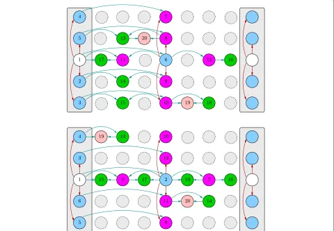
An example of two different scheduling orders is pre-sented in Fig. 6. For the sake of simplicity, only the

(10)

scheduling for the first 20 packets is presented. We observe that since clustering has been performed at pre-diction level, when Algorithm 1 is run, at step 8, any frame of a given prediction level can be selected.

In this example, we show how the algorithm could run within nodes 5 and 6 in Fig. 3. Their coding windows are depicted, respectively, in the top and bottom parts of Fig. 6. In this case, a receiver such as node 8 would see M=2 sources (or senders).

Letf(v,k)be thekth frame in display order of viewv, with the views denoted top to bottom as 1, 2,. . ., 5 so that v=3 is the central view.

In the first round, senders 5 and 6 each consider predic-tion levelL0only. As a result, they have an identical coding window containing only the I-frame of the central view— which is the only frame in the cluster of prediction level L0:W1,5 = W1,6 = {f(3, 0)}, whereWr,k is the coding

window of senderkat roundr.

In the second round, senders 5 and 6 each randomly select a frame from prediction level L1, likely a dif-ferent one. Let us, for example, assume that W2,5 = {f(3, 0),f(4, 0)}andW2,6= {f(3, 0),f(3, 4)}.

In the following rounds, both senders keep adding a ran-dom frame from the cluster of prediction levelL1to their coding windows, until no frame is left to be selected:

W3,5=W2,5∪f(5, 0) W3,6=W2,6∪f(2, 0) W4,5=W3,5∪f(1, 0) W4,6=W3,6∪f(1, 0) W5,5=W4,5∪f(2, 0) W5,6=W4,6∪f(5, 0)

Eventually, both senders will have included the whole cluster of frames of prediction levelL1in their coding win-dows, which would therefore be again identical:W6,5 = W6,6=f(1, 0),f(2, 0),f(3, 0),f(3, 4),f(4, 0),f(5, 0).

On the receiver side (node 8), let us consider the setUr

of the decodable frames received by the end of roundr. In the first round, since the coding windows of the two senders are identical, the receiver only obtains one decodable frame,U1= {f(3, 0)}.

Then, since the schedules of 5 and 6 diverge, the receiver starts obtaining on average more than one new decodable frame per round:

U2=U1∪f(4, 0),f(3, 4) U3=U2∪f(5, 0),f(2, 0) U4=U3∪f(1, 0)

Eventually, the receiver is able to decode the whole prediction levelL1(and prediction levelL0, which is com-posed of f(3,0) alone). As a consequence, the following packets received from 5 and 6 will not be innovative, meaning that they are linear combinations of the packets inU4and do not increase its rank:U6 = U5 = U4. How-ever, this redundancy is effective against packet losses.

The same algorithm is applied for subsequent prediction levels until the whole GOP is transmitted.

More in general, once the order of inclusion has been selected, each node generates a set ofNW mixed pack-ets by applying EWNC, while the original stream will be discarded. When a node receives a request from one of its neighbors to stream the content, it will answer with as many combination packets as its capacity allows. The receiver will then collect all the packets it receives from its neighbors and try to decode as many video frames as possible. It will then select a view of the content and display the relative decoded frames, achieving a video quality depending on the frames it received and the view it selected. The node will also in turn generate new com-binations to contribute to future requests.

In this description of the scheduling algorithm, we assumed for the sake of simplicity that each view frame fits in one packet. However, the algorithm is immedi-ately generalized to the case when any other data struc-ture is used, provided that it is possible to determine its rate, distortion, and coding dependencies. For exam-ple, slices could be used; or more than one frame can be included in the same packet. Given these three pieces of information, Algorithm 1 can be run on any coded data structure.

5 Experimental results

In this section, we present the results of the proposed technique and compare them with three different ref-erence techniques. The simulation scenario is the one depicted in Fig. 1 of Section 3.

The receiverRis trying to obtain the multi-view con-tent from its neighborsSm,m∈ {1,. . .,M}, referred to as

senders or sources, each connected to the receiver with a channel having capacity Cm. The channel may be a

PEC with packet loss rate εm or a GE characterized by

{εG,εB,pGB,pBG}. The receiver, at each GOP, randomly selects a view according to the probability distribution of

p. In the first experiment, we will consider a PEC chan-nel with a perfect knowledge of user preferences. Later, we will show the results when a GE model is employed and when preference estimation is not perfect.

We have selected three reference techniques to be com-pared with our proposed technique.

(11)

to the one previously proposed by the authors in [44] and is labeledEWNC in the figures.

• The second reference uses practical network coding [25] to transmit the stream. Since the senders are uncoordinated, they are not aware of the number of other senders or the capacities of their channels. Therefore, they use a coding window of the same size of the generation (i.e., the same size as the GOP). This technique is labeledPNC in the figures. In our scenario, each of the senders generates as many packets as it is the rank of the input generation, i.e., no redundancy is added by the senders. However, from the receiver side, the redundancy is inherent in havingM>1uncoordinated senders transmitting linear combinations of the same sender generation. So, in each of our scenarios, the redundancy is r=(M−1)/M.

• The last reference does not use network coding, nor it is aware of the user preferences. This technique is inspired by classical replication schemes, such as the one proposed in [47], and is labeledNO NC in the figures.

We used four common multi-view video sequences: “Ballet,” “Bookarrival,” “Breakdancers,” and “Doorflowers.” They have 1024 × 768 pixels and 25 frames per sec-ond. We used 100 frames per view and the first 5 views per sequence, for a total of 2000 frames. They have been encoded in H.264/MVC using the GOP structure described in Section 3 and depicted in Fig. 2, with QPs 31, 34, 37, and 40. The corresponding coding rates range from 280 to 1570 kbps per view. The results presented are obtained averaging over at least 100 runs and over all the sequences.

We tested the system using four models of view pref-erences. In the first one, called “peaky” distribution, the central view has a given probabilitypcand the other views share uniformly the residual probability. In a second one, called “triangular,” probabilities increase linearly from the left-most view to the central, then they decrease sym-metrical up to the right-most view. A third model uses a discrete Gaussian-like distribution, where probability of

viewk is proportional toe(k−c)

2

2σ2 _{, where}_c_{is the index of}

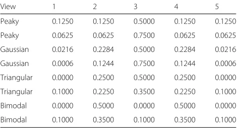
central view. Finally, we consider a “bimodal” distribu-tion where two views, symmetrical with respect to the central one, have the same probability, and the remain-ing share the residual probability. We consider at least two cases for each of the models, ending up with the probabil-ity distributions shown in Table 2. All these distributions are characterized by a single parameter, the probability of the preferred view. We refer to this parameter aspceven though in the bimodal case, this is not the probability of the central view.

Table 2View preference distributions used in the experiments

Peaky 0.1250 0.1250 0.5000 0.1250 0.1250

Peaky 0.0625 0.0625 0.7500 0.0625 0.0625

Gaussian 0.0216 0.2284 0.5000 0.2284 0.0216

Gaussian 0.0006 0.1244 0.7500 0.1244 0.0006

Triangular 0.0000 0.2500 0.5000 0.2500 0.0000

Triangular 0.1000 0.2250 0.3500 0.2250 0.1000

Bimodal 0.0000 0.5000 0.0000 0.5000 0.0000

Bimodal 0.1000 0.3500 0.1000 0.3500 0.1000

For each GOP, each user randomly selects a view according to the distribution of p, decodes the corre-sponding frames, and measures the PSNR as

PSNRw=10 log10 2552

vpvDv

(3)

that is, the distortion is the weighted MSE described in Section 4. This PSNR is reported as a function of the chan-nel capacity, which in turn is expressed as a percentage of the video stream rate.

The interesting use case is when the channel capac-ity is intermediate between a very low value (where the only possible strategy is to send the I-frame of the GOP) and high values, where any solution would work quite well. The results of these experiments are reported in the following.

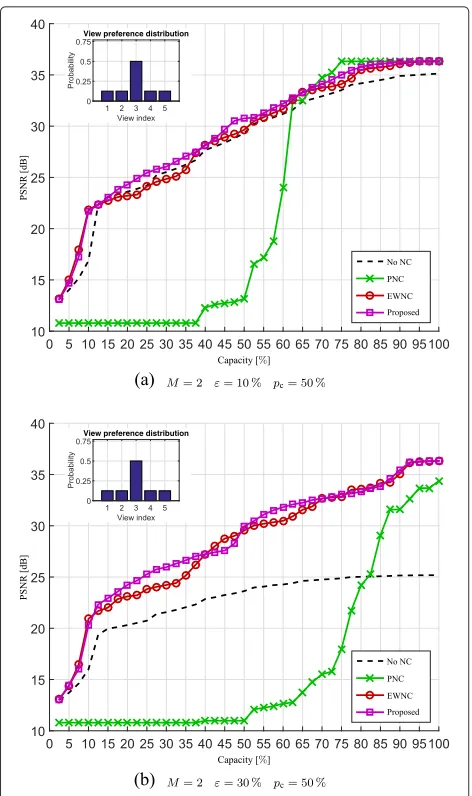
We start by considering the peaky distribution. In Fig. 7, we report a comparison with the reference techniques for a two senders’ scenario, PEC channel with packet loss rate of 10 and 30 %. The probability of the receiver displaying the central view ispc = 50 %, while the other views are equally probable.

First of all, we observe that our proposed technique out-performs all of the reference techniques for the majority of the values of channel capacity and has very similar performances in the remaining cases.

We also observe that, if no network coding is used, each received packet increases the PSNR. However, the trans-mission cannot recover from losses, thus the maximum quality is not achieved. The EWNC technique follows the same trend as the NO NC technique, but with slightly bet-ter performance, due to the effects of NC that partially compensates for the losses.

(12)

Fig. 7Comparison of the average PSNR of the decoded sequences (2 sources, 50 % probability of the receiver displaying the central view). Packet loss rates are 10 % (top) and 30 % (bottom). The capacity of the channels is expressed as a ratio of the rate of the stream. For each sequence, the PSNR is computed as the average over the views weighted by the preference probabilities as shown in the panel

is below a threshold of about 50 % of the stream rate. For higher loss probabilities, the PNC approach is even more impaired and is practically useless unless the chan-nel capacity approaches the stream rate. The necessity of a high minimum capacity to achieve any acceptable quality is a very undesirable property in a wireless envi-ronment; as in a mobile scenario, the channel conditions could rapidly become very harsh, leaving then the node with no useful data. Also, it is worth noticing that, as mentioned in Section 1, the rate of a multi-view stream can be several times larger than that of the traditional, single-view, stream. The mobile nodes are therefore likely to have an uplink capacity that is only a small fraction of the multi-view stream rate.

Table 3PSNR gain of the proposed technique with respect to the references, averaged over the channel capacity.M=2 sources, peaky distribution,Pc=50 %

ε=5 % ε=10 % ε=20 % ε=30 %

NO NC 0.86 1.10 4.95 6.08

PNC 7.16 7.76 9.93 12.29

EWNC 0.50 0.47 0.63 0.43

In Table 3, we reported the PSNR gain of the proposed technique with respect to the three reference techniques averaged along the channel capacity and for different values of packet loss probability. We observed that the proposed technique outperforms in average all the refer-ences, even though in this configuration, EWNC achieves a close performance. In the following tables from 4, 5, and 6, we show the result for similar experiments where we just change the preference probabilities. Gains are even larger for distribution other than the peaky one.

In Fig. 8, we present the results for the same number of senders and the same packet loss rates, when the prob-ability of the receiver of displaying the central view is pc = 75 %, while the other views are equally probable. We also reported in Table 7 the average PSNR gains of the proposed technique with respect to the references. Tables from 8, 9 and 10 report results for the other distributions, again in the case where the preferred view has a large probability. The proposed techniques report consistent gains in all these configurations.

As we can see both from the table and the figure, while the performance of the proposed technique and of PNC stays almost unaltered, the performance of the EWNC and of the NO NC techniques drops visibly. This can be explained by the following observations: the pro-posed technique adapts its coding window inclusion order to the distribution of the preferences, thus producing a scheduling quasi-optimal with respect to the preferences no matter what these are. On the other hand, the PNC technique imposes joint decoding of the whole generation, so the order of inclusion is irrelevant. Finally, both NO NC and EWNC do use an RD-optimized scheduler to decide their order of transmission and inclusion (respectively),

Table 4PSNR gain of the proposed technique with respect to the references, averaged on the channel capacity. Triangular preference distribution,Pc=35 %.M=2

ε=5 % ε=10 % ε=20 % ε=30 %

NO NC 0.75 1.15 5.10 6.05

PNC 7.02 7.78 9.71 12.06

(13)

Table 5PSNR gain of the proposed technique with respect to the references, averaged on the channel capacity. Gaussian preference distribution,Pc=50 %.M=2

ε=5 % ε=10 % ε=20 % ε=30 %

NO NC 1.61 1.91 5.65 5.33

PNC 7.77 8.42 10.48 11.59

EWNC 1.47 1.44 1.63 1.08

but since they do not take into account the receiver’s preferences, their estimation of the expected distortion is incorrect, resulting in a sub-optimal order. In fact, by averaging the PSNR over the views, these two models implicitly assume a uniform distribution of preferences. We can therefore expect that their performance will be the less effective the less the preference distribution resem-bles a uniform distribution, which is what we observed experimentally.

This is confirmed by using the other preference distri-butions, as also shown in Fig. 9a, b .

In conclusion, withM=2 sources, the proposed tech-nique performs largely better than PNC and NO NC, especially when the channel conditions are harsh (high loss rate, small capacity) and the preferences are skewed. It keeps a smaller gain over EWNC, around 0.5 dB when pc = 50 % and 1.5 dB when pc = 75 % for the peaky

distribution, and higher for others.

In Figs. 10 and 11, we present analogous results forM= 4 sources and forpc =50 % andpc= 75 %, respectively.

Likewise, Tables 11 and 12 present the averaged PSNR over channel capacity at several loss rates. Similar results are obtained for the other distributions. We do not report them for the sake of brevity. However, as for the previous case, the peaky distribution is the least favorable to our technique.

We observe that increasing the number of sources improves the performance of all techniques. However, the greatest effect is visible in the PNC technique as, hav-ing the largest codhav-ing window for any value of capacity, it is the one that benefits most from the diversity of the received packets. This translates in a reduction of the min-imum capacity needed to achieve an acceptable quality and the minimum capacity needed to achieve the same quality as the proposed technique (and eventually surpass

Table 6PSNR gain of the proposed technique with respect to the references, averaged on the channel capacity. Bimodal preference distribution,Pc=35 %.M=2

ε=5 % ε=10 % ε=20 % ε=30 %

NO NC 1.07 1.47 5.87 6.63

PNC 7.29 8.07 10.08 12.39

EWNC 0.38 0.46 0.50 0.19

it). These minimum capacities of course are affected neg-atively by the packet loss rates, and the range of capacities in which PNC can outperform the proposed technique narrows further when the distribution of the receiver’s preferences is less uniform (Fig. 11). Similar results are

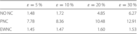
Table 7PSNR gain [dB] of the proposed technique with respect to the references, averaged on the channel capacity. Peaky preference distribution,Pc=75 %,M=2

ε=5 % ε=10 % ε=20 % ε=30 %

NO NC 1.48 1.72 4.85 6.27

PNC 7.78 8.36 10.48 12.91

(14)

Table 8PSNR gain of the proposed technique with respect to the references, averaged on the channel capacity. Triangular preference distribution,Pc=50 %.M=2

ε=5 % ε=10 % ε=20 % ε=30 %

NO NC 2.51 2.87 5.09 2.92

PNC 8.14 8.98 9.56 9.02

EWNC 2.48 2.52 1.45 0.86

obtained for the other distribution, as shown in Fig. 12. Moreover, the proposed technique still provides globally better performance than the reference ones, as shown in Tables 11 and 12. As expected, the gains are larger for less uniform preference distributions and the gain with respect to PNC increases with the packet loss ratioε.

If the number of available sources increases, the PNC approach will finally provide the best performance. In our experiments, we found that the threshold is M = 6 for a packet loss ratio ε = 10 %. However, we underline that all the parameters of these simulations (sender uplink capacities, packet loss rate, user preferences, and in par-ticular number of senders per receiver) are in general not under control of the service provider. Thus, even though there exist specific scenarios in which PNC could provide a better service than the proposed technique, the latter has a more stable and predictable behavior, much less influ-enced by these factors, and in particular by the network-dependent factors, which—in a wireless network—could change frequently and abruptly.

In Fig. 13, we show the distribution of the PSNR’s per view in the case of Gaussian preference distribution,pc=

50 %, loss rate= 10 %, andM = 2 sources. We observe that when the channel capacity is small, our technique allocates the resources to the central view, in such a way that the PSNR distribution has a behavior similar to the view preference distribution. On the contrary, the other strategies have a quite uniform per-view PSNR. Of course, when the capacity is high, all the strategies achieve very high PSNR over all the views. Lower PSNR for PNC and NO NC is explained as before, i.e., these techniques are less robust to losses.

Even though, as we stated in Section 3, the estima-tion of the preference distribuestima-tion is outside the scope of this article, it is worth mentioning the effects of an

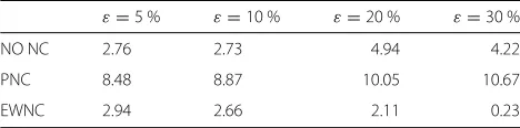
Table 9PSNR gain of the proposed technique with respect to the references, averaged on the channel capacity. Gaussian preference distribution,Pc=75 %.M=2

ε=5 % ε=10 % ε=20 % ε=30 %

NO NC 2.76 2.73 4.94 4.22

PNC 8.48 8.87 10.05 10.67

EWNC 2.94 2.66 2.11 0.23

Table 10PSNR gain of the proposed technique with respect to the references, averaged on the channel capacity. Bimodal preference distribution,Pc=50 %.M=2

ε=5 % ε=10 % ε=20 % ε=30 %

NO NC 3.05 2.49 5.29 4.58

PNC 8.57 8.63 9.04 10.38

EWNC 2.49 1.69 0.49 0.20

Fig. 9Comparison of the average PSNR of the decoded sequences (2 sources, packet loss rate 10 %). View preference distributions are Gaussian and bimodal, with maximum probabilitypcequal to 50 %

(15)

incorrect preference model on the performances of the technique. The effect on our technique is that the perfor-mance is negatively affected and becomes closer to those of the EWNC technique. Since the EWNC technique is equivalent to ours when a uniform probability model is assumed, our technique still outperforms this reference as long as the model used is a better approximation of the real distribution than the uniform model, e.g., in terms of Kullback–Leibler divergence. In order to prove this, we performed an experiment in which the proposed tech-nique uses an estimation of the central view probability, ˆ

pc ∈ {10 %, 20 %, 30 %, 50 %, 60 %, 75 %, 90 %}, while the true user preference ispc = 50 %. In order to keep

Fig. 11 Comparison of the average PSNR of the decoded sequences (4 sources, 75 % probability of the receiver displaying the central view). Packet loss rates are 10 % (top) and 30 % (bottom). The capacity of the channels is expressed as a ratio of the rate of the stream. For each sequence, the PSNR is computed as the average over the views weighted by the preference probabilities as shown in the panel

(16)

Table 11PSNR gain of the proposed technique with respect to the references, averaged over the channel capacity.M=4, Pc=50 %

ε=5 % ε=10 % ε=20 % ε=30 %

NO NC 1.22 1.32 1.20 2.63

PNC 0.95 1.78 2.46 3.60

EWNC 0.41 0.72 0.61 0.53

(i.e.,pˆc=10 %), the global performance is still better than EWNC, which corresponds to the point pcˆ = 20 %. In conclusion, even when the preference probabilities are not very precisely estimated, the proposed technique can pro-vide better performance than the reference ones, propro-vided that the estimated preferences are not much worse than the implicit estimation of EWNC.

In a further experiment, we considered two new clus-tering structures, to assess how these impact on the rate-distortion performance of the system. We used the same conditions as in Figs. 7a and 10a, i.e., peaky distribution, pc = 50 %, error probability ε = 10 %, andM = 2 or

M=4 sources.

1. In the first case, we use a larger number of clusters: this means that the labels are better representative of the clusters, but the “randomness” of the approach is limited. ForM=2sources, we found a practically identical PSNR result with respect to the initial clustering, while forM=4, we registered a very small loss (PSNR= −0.06dB). This is reasonable; having small clusters makes ineffective having multiple sources, since the senders are obliged to pick frames in the small sets.

2. In the second case, we used a smaller number of clusters, i.e., we merged prediction levels two by two. This means that we have large clusters, and the hypothesis of similar rates and distortions within a cluster is less reasonable. On the other hand, we improve the “randomness” of the algorithm. We observed slightly larger losses both forM=2 (PSNR= −0.07dB) and forM=4

(PSNR= −0.12dB); we are not able to take advantage of the improved randomness, and we pay the fact of less representative cluster labels.

Table 12PSNR gain of the proposed technique with respect to the references, averaged over the channel capacity.M=4, Pc=75 %

ε=5 % ε=10 % ε=20 % ε=30 %

NO NC 1.85 1.76 1.77 3.02

PNC 1.59 2.14 2.98 4.07

EWNC 1.42 1.52 1.54 1.46

Fig. 12Comparison of the average PSNR of the decoded sequences (4 sources, packet loss rate 10 %). View preference distributions are triangular and bimodal, with maximum probabilitypcequal to 50 %.

The capacity of the channels is expressed as a ratio of the rate of the stream. For each sequence, the PSNR is computed as the average over the views weighted by the preference probabilities as shown in the panel

As a conclusion from these new tests, we observe that the structure of the cluster has some impact on the global RD performance, related to the trade-off between rep-resentation and randomness. However, in all cases, the performance is better than the references.

(17)

Fig. 13 Average PSNR per view of the decoded sequences (2 sources, Gaussian distribution with 50 % probability of the receiver displaying the central view, packet loss rates 10 %). Channel capacities fromC=25 % toC=100 % are considered

Fig. 14PSNR vs. channel capacity when preference estimation is wrong.M=2 andε=10 %

and reference techniques are shown in Fig. 16, while the average PSNR gains are reported in Table 15. We observe results similar to those obtained for the PEC same global loss probability, for both values ofpc. Moreover, the pro-posed technique outperforms the others for practically all the values of the channel capacity. In conclusion, chang-ing the channel model does not modify a lot the rank-ing among the tested techniques, and the proposed one confirms being the best when the transmission conditions are the most difficult.

Table 13PSNR losses of the proposed technique and relative entropy of the estimated preference distribution with respect to the perfect estimationpc=50 %.M=2 andε=10 % ˆ

pc D(p||ˆp) PSNR

10 % 0.74 −1.14

20 % 0.32 −0.47

30 % 0.13 −0.23

60 % 0.03 −0.03

75 % 0.21 −0.08

(18)

Fig. 15Graph of the PSNR losses of the proposed technique vs. the relative entropy of the estimated preference distribution with respect to perfect estimationpc=50 %.M=2 andε=10 %

To summarize, we can conclude that our approach, thanks to the early decodability offered by EWNC and the a priori on the users in terms of distribution of the pre-ferred views, is able to provide both a more consistent video quality, and—in the vast majority of scenarios— better than PNC. Other approaches, such as using EWNC without exploiting the preference distribution, or not using NC at all, are always outperformed by the proposed technique. Even when the estimation of preferences is not perfect, the proposed technique is worth using, pro-vided that this estimation is not too wrong. With respect to PNC, we observe that the higher gains are achieved when the number of senders is small, the capacities of the channels are low, and the packet loss rate is high. In other words, the benefits of the proposed technique are more visible when the transmission conditions are harsher (e.g., small capacity, high error probability), which is a particularly interesting case for wireless services.

6 Conclusions

In this work, we presented a novel technique for dis-tributed video streaming of multi-view content over a wireless network. The challenge consists in transmitting a multi-view stream, with the associated high bitrate, in

Table 14Gilbert-Elliot model parameters used in the experiments

εG 10 %

εB 30 %

pGB 5 %

pBG 20 %

Fig. 16Comparison of the average PSNR of the decoded sequences (2 sources) using a Gilbert-Elliot channel model (see Table 14). The probabilities of the receiver displaying the central view are 50 % (top) and 75 % (bottom). The capacity of the channels is expressed as a ratio of the rate of the stream. For each sequence, the PSNR is computed as the average over the views weighted by the preference probabilities

a mobile network where the channel capacities are lim-ited and the packet loss rates may be high. To address this challenge, we propose to use network coding as a trans-mission technique, which—thanks to its unique property of allowing uncoordinated cooperation of the nodes—is

Table 15PSNR gain of the proposed technique with respect to the reference,M=2. Gilbert-Elliot channel with parameters in Table 14

pc=50 % pc=75 %

NO NC 3.36 3.94

PNC 8.42 9.02

(19)

able to fully exploit the available capacity. In particular, in order to dynamically adapt to the network conditions, we propose to use expanding window network coding, a net-work coding scheme that allows instant decodability of the combined packets.

In order to be able to adapt the transmission to the channel capacity, the frames are included in the coding window of each sender in an order determined by an RD-optimized scheduler. The key idea is to use the users’ preferences to identify the parts of the content more likely to be needed by the receiver in order to display its selected view. This induces a definition of the expected distortion of the stream as a weighted average of the distortion of the views. Using this metric, in order to reduce the probability of generating non-innovative packets, the senders generate a simplified probabilistic RD model that provides them with a degree of freedom in the choice of the schedule. Thus, the senders are able to generate a multitude of different, close to the opti-mum, network-coded flows that, when decoded jointly by the receiver, allow for a high and stable expected video quality.

We compared the performance of our proposed method with several techniques, in a wide range of scenarios, in terms of number of senders, channel models and capacity, user preferences, and quality of the preference estimation. We observed that the introduction of the preferences, jointly with the constraint imposed on the instant decod-ability of the selection, significantly improves the perfor-mance w.r.t. the reference techniques in the vast majority of the scenarios, in terms of video quality (PSNR) for a given capacity. Possible future work includes the develop-ment of a large-scale interactive multi-view distribution system, in particular in the direction of a joint design of an overlay management protocol that could select which nodes of the network should rely the stream. This opti-mization could be performed using topological informa-tion inferred from the packet exchanges of neighboring nodes.

Competing interests

The authors declare that they have no competing interests.

Author details

1_{DxO, Paris, France.}2_{I3S CNRS/UNSA, Sophia Antipolis, France.}3_{LTCI, CNRS,}

Télécom ParisTech, Université Paris-Saclay, 75013, Paris, France.

Received: 30 June 2015 Accepted: 12 January 2016

References

1. (F Dufaux, B Pesquet-Popescu, M Cagnazzo, eds.),Emerging Technologies for 3D Video: Creation, Coding, Transmission and Rendering. (Wiley, UK, 2013) 2. M Tanimoto, MP Tehrani, T Fujii, T Yendo, Free-viewpoint TV. IEEE Signal

Proc. Mag.28(1), 67–76 (2011)

3. P Merkle, A Smolic, K Muller, T Wiegand, Efficient prediction structures for multiview video coding. IEEE Trans. Circ. Syst. Video Technol.17(11), 1461–1473 (2007). Invited Paper

4. GJ Sullivan, JR Ohm, inProceedings of SPIE Conference on Applications of Digital Image Processing. Recent developments in standardization of high efficiency video coding (HEVC) (International Society for Optics and Photonics, San Diego, 2010)

5. A Vetro, T Wiegand, GJ Sullivan, Overview of the stereo and multiview video coding extensions of the H.264/MPEG-4 AVC standard. Proc. IEEE.

99(4), 626–642 (2011). Invited Paper

6. GJ Sullivan, JM Boyce, Y Chen, J-R Ohm, CA Segall, A Vetro, Standardized extensions of high efficiency video coding (HEVC). IEEE J. Sel. Topics Signal Process.39(6), 1001–1016 (2013)

7. H Schwarz, C Bartnik, S Bosse, H Brust, T Hinz, H Lakshman, P Merkle, K Muller, H Rhee, G Tech, M Winken, D Marpe, T Wiegand, inProceedings of IEEE Internantional Conference on Image Processing. Extension of high efficiency video coding (HEVC) for multiview video and depth data (IEEE, Orlando, FL, USA, 2012)

8. MP Tehrani, T Senoh, M Okui, K Yamamoto, N Inoue, T Fujii, in

International Organisation For Standardisation. [m31095][FTV AHG] Use cases and application scenarios for super multiview video and free-navigation, (2013). ISO/IEC JTC1/SC29/WG11

International Organisation For Standardisation. [m31103][FTV AHG] Introduction of super multiview video systems for requirement discussion, (2013). ISO/IEC JTC1/SC29/WG11

International Organisation For Standardisation. [m31261][FTV AHG] Multiple aspects, (2013). ISO/IEC JTC1/SC29/WG11

11. A Dricot, J Jung, M Cagnazzo, F Dufaux, B Pesquet-Popescu, Subjective evaluation of Super Multi-View compressed contents on high-end light-field 3D displays. Elsevier Signal Process. Image Commun.39, 15 (2015)

12. A Dricot, J Jung, M Cagnazzo, B Pesquet-Popescu, F Dufaux, inIEEE International Conference on Image Processing (ICIP). Full parallax super multi-view video coding, vol. 1, (Paris, 2014), pp. 135–139

13. SS Savas, CG Gürler, AM Tekalp, E Ekmekcioglu, S Worrall, A Kondoz, Adaptive streaming of multi-view video over {P2P} networks. Signal Process. Image Commun.27(5), 522–531 (2012).

doi:10.1016/j.image.2012.02.013. Advances in 2d/3d video streaming over p2p networks

14. C Ozcinar, E Ekmekcioglu, A Kondoz, inImage Processing (ICIP), 2014 IEEE International Conference On. Adaptive 3D multi-view video streaming over p2p networks, (2014), pp. 2462–2466. doi:10.1109/ICIP.2014.7025498 15. O Abdul-Hameed, E Ekmekcioglu, A Kondoz, inAdvanced Video

Communications over Wireless Networks. State of the art and challenges for 3D video delivery over mobile broadband networks (CRC Press, Boca Raton, FL, USA, 2013), pp. 321–354

16. C Greco, M Cagnazzo, A cross-layer protocol for cooperative content delivery over mobile ad-hoc networks. Inderscience Int. J. Commun. Netw. Distrib. Syst.7(1–2), 49–63 (2011)

17. C Greco, M Cagnazzo, B Pesquet-Popescu, Low-latency video streaming with congestion control in mobile ad-hoc networks. IEEE Trans. Multimed.

14(4), 1337–1350 (2012)

18. VK Goyal, Multiple description coding: compression meets the network. IEEE Signal Proc. Mag.18(5), 74–93 (2001)

19. P Parate, L Ramaswamy, S Bhandarkar, S Chattopadhyay, H Devulapally, in

Proceedings of IEEE Collaborative Computing: Networking, Applications and Worksharing. Efficient dissemination of personalized video content in resource-constrained environments, (Washington, 2009), pp. 1–9 20. C Gkantsidis, PR Rodriguez, inProceedings of IEEE International Conference

on Computer Communications. Network coding for large scale content distribution (IEEE, 2005)

21. R Ahlswede, N Cai, S-YR Li, RW Yeung, Network information flow. IEEE Trans. Inf. Theory.46(4), 1204–1216 (2000)

22. S-YR Li, RW Yeung, N Cai, Linear network coding. IEEE Trans. Inf. Theory.

49(2), 371–381 (2003)

23. R Koetter, M Médard, An algebraic approach to network coding. IEEE/ACM Trans. Networking.11(5), 782–795 (2003)

24. T Ho, M Médard, J Shi, M Effros, DR Karger, inProceedings of IEEE International Symposium on Information Theory. On randomized network coding, (Kanagawa, 2003)