Scaling Complex Analytical Processing on Graph Structured Data Using Map Reduce

(1)

ABSTRACT

SRIDHAR, RADHIKA. Scaling Complex Analytical Processing on Graph

Structured Data Using Map Reduce. (Under the direction of Dr Kemafor Anyanwu.)

Efficient analytical processing at the Web scale has become an important

requirement as more decision support applications rely on the data on the Web.

One approach for achieving the significant scalability is by the use of parallel

processing techniques on a computational cluster of the commodity grade

machines. Software platforms such as Map-Reduce, Hadoop and Pig are now

available that allow the users to encode their tasks in terms of simple low-level

primitives that are easily parallelizable. Further, a high-level dataflow language

called the Pig Latin has been proposed for specifying analytical processing

tasks using a mixture of the procedural and the declarative paradigms. This

approach strikes a good balance between customizability and the potential for

an automatic query optimization. However, the analytical processing capability

currently offered by these frameworks is fairly basic and as such has narrow

applicability to many real world scenarios. Furthermore, an increasing amount

(2)

documents. However, such data is typically organized as a set of binary

relations (a graph) whereas these frameworks are primarily targeted at

processing the data structured as n-ary relational tables.

This thesis addresses the problem of enabling the scalable analytical data

processing on the RDF datasets. Its approach is based on extending Yahoo’s

Pig system (an open source parallel processing) with constructs that allow

complex data processing problems on the graph structured data to be

expressed in a manner that is more amenable to automatic parallelization.

Specifically, it makes the following contributions:

1. Extends Pig Latin, the dataflow language for Pig, with primitives that

support the expression of queries in terms of a readily parallelizable

multidimensional join operator, as well as support the expression of

graph navigational filter expressions.

2. Implements the introduced primitives in a Hadoop implementation

running on VCL

(3)

Scaling Complex Analytical Processing on Graph Structured Data Using Map Reduce

by

Radhika Sridhar

A thesis submitted to the Graduate Faculty of

North Carolina State University in partial fulfillment of the

requirements for the Degree of Master of Science

Computer Science

Raleigh, North Carolina

2009

APPROVED BY:

_________________________ _________________________ Dr. Tao Xie Dr. Xiaosong Ma

________________________________

(4)

DEDICATION

(5)

BIOGRAPHY

Sridhar, Radhika was born on February 15, 1983 in Bangalore, India. She

obtained her Bachelor‟s degree in Information Science and Engineering at

Dayananda Sagar College of Engineering an affiliate of Vishweshwaraiah

Technological University, in May 2005. At the time of writing this, she was

working towards her M.S. in Computer Science at the North Carolina State

(6)

ACKNOWLEDGEMENTS

I would like to thank my advisor, Dr. Kemafor Anyanwu for her guidance, helpful

suggestions and support in completing this thesis work. I also extend my

gratitude to my committee members, Dr. Tao Xie and Dr. Xiasong Ma for their

suggestions and valuable comments during the course of my thesis.

I am highly grateful to my family and friends for all their encouragement and

support. I would have never come this far without their moral support. I would

also like to thank the Semantic Computing Research Group at North Carolina

State University for their feedback and suggestions. Special thanks to my

friends Padmashree Ravindra and Suchetha M. Reddy for their suggestions

(7)

LIST OF TABLES

Table 1 : Relational Representation of the Sales relation ... 13

Table 2 : RDF representation for the Sales relation ... 14

Table 3: ProdBought ... 16

Table 4: Price ... 16

Table 5: Location ... 16

Table 6: Fact table representing the Sales data ... 28

Table 7: Base table created for the table in the fact table ... 28

Table 8: Base table being updated with the values obtained after performing the aggregation operation ... 29

Table 9 : Data expressions in Pig Latin... 37

Table 10: Shows the result obtained after executing GFD ... 53

Table 11 : Subset of the result generated after the GBD operation ... 55

Table 12 : The results generated after the MDJOIN operation ... 58

Table 13: Cost analysis for the query execution on BSBN dataset ... 75

(11)

LIST OF FIGURES

Figure 1: Graphical view of the simple RDF statement ... 9

Figure 2: Graphical representation of the Sales data ... 13

Figure 3 : The architecture of Map-Reduce framework ... 31

Figure 4: Pig Latin architecture ... 35

Figure 5: Pseudo code for Map Function ... 41

Figure 6: Pseudo code for Combiner Function ... 42

Figure 7: Pseudo code for Reducer Function ... 44

Figure 8: Execution on GFD for Example 4.1 ... 52

Figure 9: Execution of the GBD for the Example 4.1 ... 55

Figure 10: Execution of MDJ for Example 4.1 ... 57

Figure 11: Architecture of Pig Latin Language ... 67

Figure 12 : Execution plan of GBD and GFD on Map-Reduce ... 69

Figure 13 : Execution plan for MDJ on Map-Reduce ... 69

Figure 14: Example subgraph taken from the BSBM dataset ... 72

Figure 15: Graph shows the cost analysis using the two approaches ... 78

Figure 16: Example subgraph taken from the DBLP dataset ... 79

Figure 17: Graph shows the cost analysis using the two approaches ... 83

Figure 18: Screen shot of the Manage Images page ... 98

Figure 19: Screen shot of the Create an Image page ... 99

Figure 20: Screen shot of the Connect page ... 100

Figure 21: Screen shot of the new Reservation page ... 102

(12)

Figure 24: Screen shot of the sample input data file ... 109

(13)

LIST OF ABBREVIATIONS

BSBM : Berlin SPARQL Benchmark

DBLP : Data Base systems and Logic Programming

GFD : Generate Fact Dataset

GBD : Generate Base Dataset

MDJ : Multi-Dimensional Join

N3 : Notation 3

OLAP : On-Line Analytical Processing

RDF : Resource Description Framework

SPARQL : Simple Protocol And RDF Query Language

SQL : Structured Query Language

SWETO : Semantic WEb Technology evaluation Ontology

UDF : User Defined Function

URI : Uniform Resource Identifier

WWW : World Wide Web

W3C : World Wide Web Consortium

(14)

Chapter 1 Introduction

Structured data now constitutes a growing segment of the data being made

available on the Web. This trend is due to more organizations appreciating the

advantage of making their data available on the Web and also because of the

increasingly popular mechanisms for annotating Web content with metadata.

These annotation mechanisms range from the informal methods used by

applications such as Flickr [12], Delicious[14] Google Co-op[13] that allow users

“tag” digital resources with tags of their choice, to the more formal

representation schemes such as Microformats, XHTML, Resource Description

Framework (RDF)[15], RDF in attributes (RDFa),` Rich/RDF Site Summary

(RSS) etc which offer more systematic methods and languages for representing

(15)

metadata exchange on the Web, are gaining broadening adoption because of

the promise of potentially enabling reuse, exchange and automatic processing

of data. This has created an affinity for RDF in different communities,

particularly in scientific research domains where the exchange and sharing of

data and the possibility of semi-automatic data integration support is highly

desirable. One of the Semantic Web search engines, SWOOGLE[26], now

reports that there are several millions of RDF documents currently available on

the Web. The implication of this is that, while on the current Web, documents

marked up with tags that improve the presentation of the document content to

enable human understanding, the Semantic Web will have documents in which

machines will be able to understand the content on the Web and perform tasks

on behalf of users. Further, current generation data processing techniques for

the Web will need to be advanced to deal with the structure and semantics in

the new Web. In particular, techniques that support more analytical tasks as

opposed to the traditional searching and fact-finding will need to be developed

for supporting communities such as scientific research communities.

1.1 Analytical Processing

(16)

processing of queries demanding aggregations over multidimensional

groupings of data. In OLAP, numeric facts about the data called measures are

represented collectively in a table called the fact table and every measure is the value of the attribute associated with the data. Attribute are categorized by a

dimension that is derived from the dimension tables. The dimension provides information about the measure or the attribute. In OLAP, queries aggregate

subsets of values in the fact table along multiple dimensions. For example,

Assume that we have a Customer relation (CustID, CustName) (typically called

a dimension table), a Sales relation (CustID, ProdID, Price, Location) (typically

referred to as a fact table) that relates customers to products that they bought and the price paid and location in which the sale occurred. We may want to compute total sales amounts when grouped by all combinations of product,

month and state. This results is a query with aggregations (total sales) over eight different groupings for every combination of product, month and state (i.e.

none, (product), (month), (state), (product & month), (month & state), (state & product) and (product & month & state). Such queries are fundamental to

analytical tasks in business and financial applications. However, investigative

applications such as in scientific research domains, often require more ad-hoc

analytical queries as well as scientific research domains but are challenging

(17)

such as the CUBEBY, ROLLUP, etc were added to SQL which makes

reporting-style queries. However, ad-hoc analytical queries tend to be more

complex and are not easily expressible they require multiple aggregations over

different groups. For example, suppose we want to gain some insight into the

buying patterns in a particular region, we might want to compute for every

customer, the total amount of their purchases in either of the states, say “NY” or “NJ”. This is called a “pivoting” query whose result is a relation (CustID,

Total_NY, Total_NJ). Since this requires computation of sales in those states for every customer. Expressing such queries using traditional relational

database approach would require two subqueries (one for each location) to

compute the total amount of sales for the location, then two outer joins to

Customer table to assemble the final result. Such a query expression is

cumbersome and optimizers don‟t often select the best execution plan for them.

Consider the Sales schema shown below [7]:

Sales(CustID, ProdID, Price, Location, Month, Year), to compute the

average for each customer who purchased the products in “NY’, “NC”

and “NJ”.

Evaluating such a query using the regular relational database operator would

(18)

customer sales in NY, NC and NJ respectively. The result gives a list of all the

customers, whether or not they made any purchases in these states. We need

another subquery to select all the unique customers. Finally, we need four outer

joins to attach the sales to the customers in NY, NC and NJ locations.

A key observation made in [7] is that, there exists a tight coupling between the

grouping operations and the aggregation function that needs multi-pass

aggregation.

1.2 Challenges of Analytical Processing on RDF

Scalability - The issue of efficient processing of data at Web scale is still a primary concern for search engine companies as datasets range to terabytes of

data. Parallel processing seems to be one promising approach for processing

data at a Web scale. Traditional approaches that use high-end parallel

database systems with highly specialized architectures such as Teradata,

Tandem, NCR, Oracle-n CUBE, and RAC or OLAP servers such as Microsoft

OLAP servers, SAS OLAP server are not cost effective and easily adoptable

strategy. These high end systems, though quite capable of handling data stores

at enterprise scale, are not designed for the Web scale processing and are too

expensive to be a practical alternative for supporting the Web scale processing.

Alternatively, there are leading efforts to develop platforms that enable parallel

(19)

Google, is the Map-Reduce [18] framework that has its roots in functional

programming languages. Further, Apache‟s release of an open source version of Map-Reduce called Hadoop [1] derive from the Map-Reduce approach. These platforms are designed to run parallel programs on a computational

cluster of commodity grade machines, a paradigm popularly known as cluster computing. Further, a language Pig Latin [6] is built on top of Hadoop which is

an open source implementation of the Map-Reduce Framework. Pig Latin is an

algebraic dataflow language that expands the scope of primitives to enable the

reuse of common code fragments and provides the opportunity for applying

query optimization techniques. However, these approaches currently focus on

supporting the simple data processing tasks with the limited support for semi

structured or graph structured data such as RDF.

In order to execute ad-hoc queries on RDF datasets, before performing any

aggregation operations, we need to reassemble all the tuples with the related

predicates. A series of join operations are required to reassemble the tuples.

After reassembling the tuples, multi-pass aggregations need to be computed

which requires repeated processing on the same set of tuples with slightly

different computations, thus making the execution of these queries inefficient.

Our aim is to provide an efficient approach that can perform analytical querying

(20)

Various operators like the MD-Join, GMD-Join are proposed in the relation

database to perform efficient complex analytical query executions.

There are various areas that require performing analytical queries on the

Semantic Web. Fields like biomedical research, bioinformatics, etc., aim in

turning Semantic Web into practical applications that involve performing

complex analytical queries on the data to enhance the research ideas leading to

new innovations and discoveries

With such rapid growth rate of the semantic data, there is an increasing need

for a scalable approach to process these data. There are various scalable

parallel processing approaches like the Map-Reduce framework, Pig Latin

language that executes over a Map-Reduce framework and so on. But these

approaches currently process simple data efficiently. Executing complex

analytical queries on structured semantic data using these frameworks are yet

to be researched.

1.3 Data processing on the Semantic Web

A fundamental data model for the Semantic Web is called the Resource Description Framework (RDF) [15] . In RDF, a simple statement is a triple of the

(21)

subject and the Object holds the value for that property. The triple

representation of RDF can be used to describe any concept, relationship or an

object that exists in the universe. In RDF the resources are identified using

simple Web identifiers called the Uniform Resource Identifiers (URI). This

enables to represent resources and their properties as graphs of nodes and

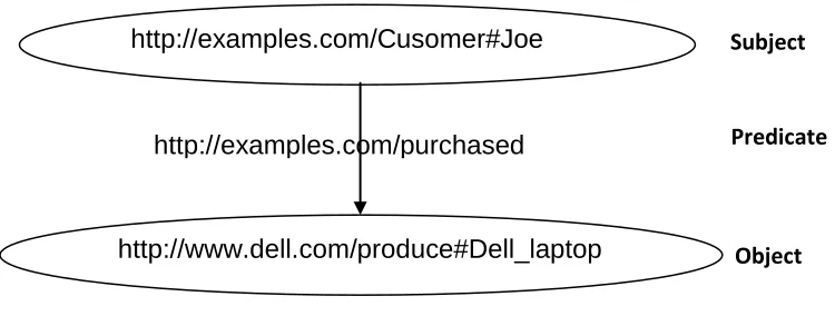
arcs representing their properties. For example, consider a general statement:

“Customer Joe purchased a Dell laptop”. The RDF representation of the

statement is as shown below:

< http://examples.com/Cusomer#Joe,

http://examples.com/purchased,

http://www.dell.com/produce#Dell_laptop >

In the above example, “http://examples.com/Cusomer#Joe” represents the

subject, “http://examples.com/purchased” represents the property and the object is represented by “http://www.dell.com/produce#Dell_laptop”. The RDF

statements can also be represented as a labeled graph connecting resources

where the labeled edges represent the properties between the resources.

(22)

Figure 1: Graphical view of the simple RDF statement

Further, RDF is a conceptual model with different serialization formats. Some

concrete formats of representation are: XML RDF, Notation 3, N-Triples, and so

on. In this section we briefly describe the Notation 3 syntax that is one of the

simplest and widely used formats of RDF representation [26]. In this notation,

the subject, predicate and the object are URI‟s enclosed with in “<” and “>”

symbols. The end of each line or a triple is denoted by “

.

”. The syntactical form

of Notation 3 is as shown below, where subject, predicate and object are atoms.

An atom can either be an URI, an URI abbreviation, a blank node or a literal.

<subject><predicate><object> .

Subject

Predicate

Object http://examples.com/purchased

http://examples.com/Cusomer#Joe

(23)

For example,

1) <http://example.org/#Joe> <http://example.org/#Type> <http://example.org/#Customer> .

2) <http://example.org/#PO12> <http://example.org/#loc> <http://example.org/#NC> .

3) <http://example.org/#PO12> <http://example.org/#price> <35>

.

Representing the data using such RDF syntax provides some structure for the

contents on the Web that makes the Web appear as a globally linked database

of triples as opposed to just a network of unstructured documents. This

provides an environment for the Web contents to be queried and analyzed to a

degree similar to what has been achieved with structured data. For example,

Search engine companies are actively investigating on techniques for analyzing

the massive amount of search log, click stream and web graph data that they

collect.

The World Wide Web Consortium (W3C) recommends SPARQL Protocol and RDF Query Language (SPARQL) [16] for querying RDF data. The SPARQL language supports querying RDF graphs and is designed to execute queries

(24)

SPARQL are represented using symbol “?” or “$” that prefix the variable name.

For example, consider a RDF statement as shown below:

<http://example.org/#PO12> <http://example.org/#price> <35> .

A query to find the price of Product PO12 can be written in SPARQL as:

SELECT ?price

WHERE {

<http://example.org/#PO12>

<http://example.org/#price> ?price . }

The result of the above query returns value 35. Simple queries can be executed

using the SPARQL query language. More complex queries can be formed by

combining multiple triple patterns to form graph patterns using combination

operators. Currently, it is not possible to express queries that require grouping

and aggregations operations using SPARQL because the language does not

support these operations. . Some systems like OpenLink Virtuoso [30], ARQ [4]

, etc., extend SPARQL with SQL like aggregate and grouping functions.

However, even with such systems in these systems, executing complex queries

does not result in efficient results. Since, queries with multiple groupings and

(25)

grouping attribute to be executed as a separate subquery. Hence each

subquery requires scanning the table at least once. Performing multiple scans

result in expensive computations.

Further, the structure of the RDF data creates some challenges in performing

complex queries on the Web content. The challenges being an n-ary tuple in a

relational scheme contains all related data values in a single unit. Thus each

tuple is independent of the other within the input file. Grouping and aggregation operations are executed on these tuples which means that such operations are

performed at the level of related data values. However, when we consider the

RDF data model, each tuple is a combination of the subject, predicate and the

object. Thus an n-ary relational tuple would be spread across a set of (n-1) RDF

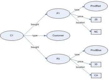
triples. For example, Figure 2 shows the graph representation for two tuples of

(26)

Figure 2: Graphical representation of the Sales data

Representing this graph in a relational database will result in a table having

attributes Customer, ProdBought, Price and Location. The data in Table 1 corresponds to the data in the graph.

Table 1 : Relational Representation of the Sales relation

Customer ProdBought Price Location

C1 P1 25 NC

(27)

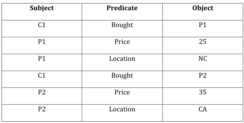
The equivalent RDF representation for the same data is shown in Table 2.

Comparing Table 1 and 2, we see, a single tuple with four attributes in the

relational representations is shredded into three tuples of subject, predicate and

object in the RDF representation.

Table 2 : RDF representation for the Sales relation

Subject Predicate Object

C1 Bought P1

P1 Price 25

P1 Location NC

C1 Bought P2

P2 Price 35

P2 Location CA

Due to the shredding of the tuple in the RDF representation, operations like

grouping or aggregation will require intensive self-joins over the same set of triples, resulting in additional cost during query executions. For example,

consider a simple query –

(28)

Expressing the above example in relational algebra:



Customer (



Location = “NC” (Sales))

In order to obtain the same result from the RDF dataset, we need to express

the above example in relational algebra as:



subject (R R.subject = S.object S)

Where,

R =



predicate = “Location and object = “NC”(Sales)

S =



predicate = “bought”

(Sales)

Further, a popular approach for efficient management of the RDF data is

commonly known as the

vertically partitioned approach,

in which the dataset

containing the RDF data is partitioned into “n“unique datasets based on the

distinct tuple properties. Every dataset contains all the tuples corresponding to

one unique property. In this approach, the tuples are still shredded, but are

stored in separate files based on their properties. Thus performing any

operations on these datasets still requires reassembling of the data, but in this

(29)

on different datasets, rather than the self join operation performed as in the

earlier approach. For example,

Consider the above examples, suppose the Sales data shown in Table 2 is

partitioned using the vertically partitioning approach, than the Sales data would

be represented as follows:

Table 3: ProdBought

Subject Object

C1 P1

C1 P2

Table 4: Price

Subject Object

P1 25

P2 35

Table 5: Location

Subject Object

P1 NC

P2 CA

Table 3 represents the data that has predicate value ProdBough. Similarly

Table 4 contains all the data that has predicate value Price and Table 5 contains data with predicate value Location. In order to obtain the same result on the vertically partitioned RDF dataset the query shown in the above

example, we can represent the query in relational algebra as follows:



_subject(R R.object = S.subject S)

Where,

(30)

S =



predicate = “bought”

(Sales)

The above example shows the need to reassemble the related RDF tuples before executing any queries on them. Table 2 also shows how the RDF format,

combines data and metadata within their representation. The attributes

ProdBought, Price and Location in the Table 1 is the actual data in the RDF dataset. This adds additional complexity in querying RDF data, since it is

necessary to check for the correct predicate before computing any aggregation

or grouping operation. These challenges show the need for an approach to

query the RDF data that is similar to the relational database queries considering

the structure of the RDF datasets.

1.4 Research Motivation

Enable analytical querying on RDF datasets:

Ad-hoc analytical queries tend to be more complex as they require multiple

aggregations over different groups or viewing the results from different

dimensions. For example [7],

(31)

Sales(CustID, ProdID, Price, Location, Month, Year), Suppose, to

compute the average sales value of each customer who purchased the

products in “NY’, “NC” and “NJ”.

Evaluating such a query using the regular relational database operator would

primarily require executing the three subqueries, each query to compute the per

customer sales in NY, NC and NJ respectively. The result gives a list of all the

customers, whether or not they made any purchases in these states. We need

another subquery to select all the unique customers. Finally, we need four outer

joins to attach the sales to the customers in NY, NC and NJ locations. This

example shows the need for multi-pass aggregation. In order to execute ad-hoc

queries on RDF datasets, before performing any aggregation operations, we

need to reassemble all the tuples with the related predicates. A series of join

operations are required to reassemble the tuples.After reassembling the tuples,

multi-pass aggregations need to be computed which requires repeated

processing on the same set of tuples with slightly different computations, thus

making the execution of these queries inefficient. Our aim is to provide an

efficient approach that can perform analytical querying efficiently on semi

(32)

A scalable approach for RDF data processing: The issue of efficient processing of data at Web scale is still a primary concern for search engine

companies as datasets range to terabytes of data. Parallel processing seems to

be one promising approach for processing data at a Web scale. Traditional

approaches that use high-end parallel database systems with highly specialized

architectures such as Teradata, Tandem, NCR, Oracle-n CUBE, and RAC or

OLAP servers such as Microsoft OLAP servers, SAS OLAP server are not cost

effective and easily adoptable strategy. These high end systems, though quite

capable of handling data stores at enterprise scale, are not designed for the

Web scale processing and are too expensive to be a practical alternative for

supporting the Web scale processing. Alternatively, there are leading efforts to

develop platforms that enable parallel processing of Web data. The winning and

popular approach, pioneered by Google, is the Map-Reduce [18] framework

that has its roots in functional programming languages. Further, Apache‟s

release of an open source version of Map-Reduce called Hadoop [1] derive from the Map-Reduce approach. These platforms are designed to run parallel

programs on a computational cluster of commodity grade machines, a paradigm

popularly known as cluster computing. Further, a language Pig Latin [6] is built

on top of Hadoop which is an open source implementation of the Map-Reduce

(33)

of primitives to enable the reuse of common code fragments and provides the

opportunity for applying query optimization techniques. However, these

approaches currently focus on supporting the simple data processing tasks with

the limited support for semi structured or graph structured data such as RDF.

1.5 Research Contributions

In the earlier section, we have discussed the issues and the challenges

involved in analytical querying on RDF datasets. Based on these challenges,

we aim to contribute the following-

 Clearly introduce the problem of analytical data processing on RDF

datasets

 Propose an approach for achieving the scalable processing of the

non-trivial analytical tasks on RDF datasets that is based on an

efficient multidimensional query operator called the MD-Join and

parallel query processing on an extended Map-Reduce framework.  Propose an approach for implementing the multi-dimensional join in a

Map-Reduce framework

 Propose an extension to the Pig Latin dataflow language that

includes the structural and semantic query expressions that are

(34)

reassembling related RDF data values and define the inputs

necessary for MD-join operator. Further, we show how this extended

Pig Latin language compiles into the Map-Reduce workflows with the

enhanced MD-joins.

1.6 Outline of the thesis

- Chapter two discusses the challenges involved in expressing the complex analytical queries and introduces the existing

multi-dimensional join operator. Further in this chapter, various

parallelism approaches for data processing are discussed.

- Chapter three discusses in detail the implementation of the multi-dimensional join operator on a Map-Reduce execution framework.

- Chapter four explains how Pig Latin language can be extended to provide new operators that can perform analytical processing on

RDF

- Chapter five discusses the execution plan for these extended operators in terms of the Map-Reduce functions

(35)

- Chapter seven discusses the related work and chapter eight highlights the possible future work.

(36)

Chapter 2

Preliminaries

2.1 Expressing Complex Analytical Queries using MD-Join

In the examples seen in section 1.1, we have observed that the complex ad-hoc

queries involve multiple aggregations over different sets of grouping values. In

the relational database, to perform a set of aggregation operations on different

grouped attributes, every aggregation operation has to be performed on one set

of grouping attributes independently and then these results have to be

combined. This tight coupling between the aggregation function and the

grouping attributes results in a series of join and union operations. The multiple

(37)

Example 2.1 - we would like to compute the total number of products

having sales between the average sale of the previous month and the

average sale of the next month, for all combinations of the product and

the month for the year “2000”.

Evaluating such a query using traditional database operators would mean to

filter out all records for which the condition year = 2000 is not valid. For tuples

where the filter condition is true, a GROUPBY operation is performed over all the

product and month combinations. We would then need to compute aggregates from tuples that are outside of each group (the previous and next month‟s

average sale). Using these results, the final aggregation value can be

computed. This example shows how cumbersome it is to express such

complex queries using the ordinary SQL operators. New operators like CUBEBY,

PIVOT, etc cannot be used in these queries as the computation is more complex than a simple aggregation over multi-dimensions. These observations

were made in [8] and an operator, the MD-Join operator, that allows the queries

to decouple the grouping and the aggregation functions, was proposed. In this

operator, a Base table is constructed, that is a container table holding all the

(38)

The actual data in the relational table represents the fact table. The following is

a formal definition for the MD-Join operator:

Definition: Let B and R be relations, Θ is a set of conditions involving

the attributes of B and R, l is a list of aggregation functions that needs

to be computed, l = (f1, f2, f3,…..fn) over attributes c1, c2, c3…,cn of R. We

define a new relational operator between B and R, called MD-Join,

defined as:

MD (B, R, l, Θ)

is a relation with schema B, f1_R_c1, f2_R_c2, ….,

fn_R_cn, whose instance is determined as follows. Each tuple b



B

contributes to an output tuple B, such that:

 Table B is augmented with as many columns as the number of

aggregate functions in l. Each column is named as fi_R_ci, i = 1,. .

. ,n

 For each row r of table B we find the set S of tuples in R that

satisfy Ɵ with respect to r, i.e. when B’s attributes in Ɵ are

(39)

column fi_R_ci of row r is the fi(ci) computed over tuples of S, i =

1,. . . ,n.

B is the base table created and R is the fact or detail table that holds the collection of related tuple values e.g. the Sales relation. The semantics of the

MD-join operator is designed in such a way that the sequence of MD-joins can

be combined together, thus making the execution of complex ad-hoc query cost

efficient.

Expressing the above example using the MD-join operator we get:

MD(MD(MD(B, Sales, AVG(sale), Ɵ1), Sales, AVG (sale), Ɵ2),Sales, AVG (sale), Ɵ3)

Where Ɵ1 : Sales.cust = cust and Sales.state= “NY”,

Ɵ2 : Sales.cust = cust and Sales.state= “NJ”,

Ɵ3 : Sales.cust = cust and Sales.state= “NC”,

And B is the table generated using a simple query of the kind, “select distinct cust from sales”.

The above example shows how the analytical query can be executing without

(40)

The MD-join operator separates the tight coupling that exists between grouping

and aggregation attributes and hence makes the query execution efficient. Due

to this separation, it is possible to compute the aggregation value for all

combination of the attributes at once instead of performing the aggregations for

each combination of attributes separately which will require additional scanning

of the table.

Algorithm:

Scan R, and for all tuples t in R{

For all rows r of B, check if condition

Ɵ is satisfied with respect to r and t.

If yes, update r‟s aggregate columns

appropriately.

}

The above algorithm shows the computation of the MD-join operator. This

operator captures the semantics of the user‟s need, more accurately as shown

in the above example. To understand the execution of the MD-join algorithm

consider the following tables. Table 6 is the fact table consisting of the Sales

(41)

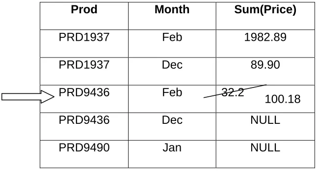
Table 8 shows the result generated after the execution of the MD-Join operator

on the fact table. When a match is found between the fact and the base table

the corresponding aggregation is computed and the value is updated in the

base table as shown in Table 5.

Table 6: Fact table representing the Sales data

Cust Prod Month Year Price

1290 PRD1937 Feb 2008 1982.89

1291 PRD9436 Dec 2007 899.98

Table 7: Base table created for the table in the fact table

Prod Month

PRD1937 Feb

PRD1937 Dec

(42)

Table 8: Base table being updated with the values obtained after performing the aggregation operation

Prod Month Sum(Price)

PRD1937 Feb 1982.89

PRD1937 Dec 89.90

PRD9436 Feb 32.2

PRD9436 Dec NULL

PRD9490 Jan NULL

2.2 Analytical data processing using parallelism approaches

2.2.1 Map Reduce Framework

Map-Reduce is a programming model designed to perform distributed

computation on clusters of computers. This framework is designed on the idea

of the functional programming technique, where the computation of the tasks is

performed by various functions. This framework defines two basic primitives

(43)

function which performs any kind of computation or aggregation operation on

the groups. These Map and the Reduce functions are simple function

prototypes which needs to be implemented by the users as per the user

requirements. To use this paradigm for data processing, tasks need to be

mapped into the Map and the Reduce functions. Data processing using this

framework is particularly suited for tasks that can be casted as

group-by-aggregation. The execution of the tasks in the map and reduce functions are

independent of each other as each of these functions perform one specific task.

Hence these functions can be executed on different processors at different

times. This allows the processing of the tasks in these functions to be

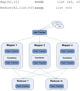
parallelized. Figure 3 shows the architecture of the Map-Reduce framework.

The framework consists of one master process and multiple task processors

running in parallel to perform either a Map function or a Reduce function. The

master process accepts the input data and splits the data into smaller chunks

and assigns each chunk to one of the available processors. The map function

reads each line in the data, generates a key and returns the result as a <key,

value> pair. After all the map processors have completed their tasks, the master function assigns the tasks for the processors to perform the reduce function.

This function sorts and merges all the intermediate keys generated by the map

(44)

computed can be performed in the reduce function. The keys and the type of

values generated for the map and the reduce functions are of the following

types:

Map(k1,v1) list (k2, v2)

Reduce(k2,list(v2) list (v2)

(45)

Consider a simple example from [18] that counts the number of occurrences of

each word in a large document using the Map-Reduce framework. The master

process reads the input file, breaks it into chunks of smaller size and assigns

the chunks to the available processors to execute the Map function. Each

processor performing the Map function receives the <key, value> pair where the

file name is the key and the file data is the value in this case.

In each map process, the data is read and the output is a list of <key, value> pairs, where the key is all the words present in the document and the value is

assigned as “one”. The processors performing the reducer function, will receive

<key, a list of value> pairs. We can now add up all the values corresponding to a key and return the number of times that key (i.e. the word) occurs. Hence the

output of the reducer will be the list of all the keys and the number of

occurrences of the word in the document. This example shows how we can

parallelize the simple task of counting the number of occurrences of each word

in a file. However, more complex processing can be achieved by customizing

the map and the reduce functions.

Further, the Map-Reduce framework is designed to work with a single dataset.

However, in many situations it is required to perform join operations over two or more data sets. The method for bypassing this limitation of a single dataset

(46)

approach, we first perform a map function, skip the reduce function but

generate the keys such that in the next cycle of map all the related data have

the same key. This approach requires one additional cycle of Map-Reduce data

flow for each of the JOIN operations performed. The other alternative is to generate a flag representing each dataset. Based on this flag we can perform

the JOIN in the reduce function. This is known as the Reduce-Side Join. These two approaches to perform JOIN operations are not very efficient because they

require an additional map and reduce phase in order to perform the JOIN

operation. Hence an extension of the Map-Reduce framework is the Map-Reduce-Merge [12] framework. In this programming model, an additional merge

phase is added, where the JOIN operation is performed between the two sets of the data that are obtained from the two different Map-Reduce cycles.

2.2.2 Pig Latin language

Map-reduce programming model has proven to be an efficient approach for the

data processing task, but with a few limitations such as:

 Rigid data flow between the Map and the Reduce functions. In the

above section, we observed, when implement the Map-Side join we

(47)

the Reduce function. We cannot eliminate this Reduce function due to

the rigid data flow between the two functions. Hence we execute the

Reduce function after the execution of the Map function but perform no

operation in the Reduce function.

 Framework‟s primary reliance on the customized functions that provide

limited opportunity for an automatic optimization and reuse of the code.

These limitations are the motivation for the development of the new dataflow

language known as the Pig Latin. The main goal of the Pig Latin language was

to achieve a sweet spot between the declarative style of the languages like SQL

and the low level procedural style of the Map-Reduce programming. In order to

achieve this, Pig Latin provides a set of predefined functions and query

expressions that can be used to describe the data processing tasks. Along with

these pre-defined functions, the language also allows the user to define their

(48)

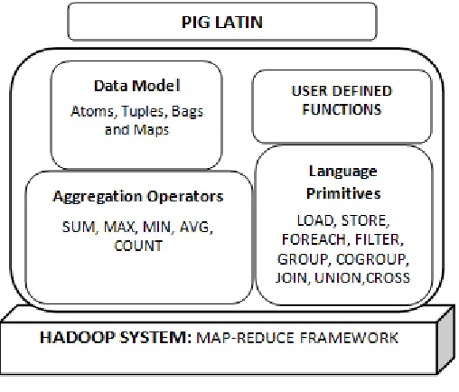
Figure 4: Pig Latin architecture

The data model for a Pig Latin consists of an atom that holds a single atomic value, a tuple that holds a series of related values, a bag that forms a collection of the tuples and a map that contains a collection of the key value pairs. A tuple

can be nested into an arbitrary depth. The basic primitive functions of the Pig

(49)

records within a given data set. The COGROUP operator is similar to the GROUP operator but focuses on grouping together the similar data from different data

sets. The JOIN function is used to merge the data from two different datasets. Other common commands similar to the SQL commands are the UNION,

DISTINCT, ORDER, CROSS, AVG, SUM, MIN, MAX and so on. STORE is used to get the results stored in an output file. In addition to these primitive, Pig Latin

provides a library of UDF‟s – User Defined Functions. The limitation of UDF is that the users will be responsible for the efficiency of their programs and they

have to specify how the functions have to be parallelized.

For example, consider the Sales schema discussed in chapter 1,

Compute the average sales within each location, where the number of

purchases in that location is greater than 3. A Pig Latin program for this

scenario, using the above mentioned operators is as follows:

groups = GROUP Sales BY Location;

group_count = FILTER groups BYCOUNT(*) > 3;

(50)

The above example shows the sequence of steps in a Pig Latin program, which

is much like any programming language. Each line in the program performs a

single data transformation. These transformations in every step are fairly high

level, resembling the SQL, e.g. FILTER, GROUP, etc. Along with these SQL like operators, Pig Latin provides a wide variety of data expressions and different

kinds of nested tuples for the data storage. This language provides a flexible

approach for accessing the data from these nested tuples. For example,

consider a tuple t with fields‟ f1, f2 and f3, where t is defined as shown below:

t = ′𝐶𝑢𝑠𝑡1′_, ′𝑁𝐶 ′_{, 25}

′𝐶𝐴′_{, 35} , ′𝑃𝑟𝑜𝑑123′

Table 9 : Data expressions in Pig Latin

Expression Type Example Value for t

Field by position

$2 ‘Prod123’

Field by name f1 Cust1

Projection f2.$1 (25)

(35)

Function Evaluation

(51)

Table 9 shows some examples of the expression type in Pig Latin and also how

these expressions operate. The flexibility provided in these expressions allows

(52)

Chapter 3 Implementing MD-join in Map-reduce

In section 2, we briefly defined the MD-JOIN operator and its advantages over

the other OLAP operators like CUBEBY, GROUPBY and so on. In this section, we

describe how the MD-JOIN algorithm can be implemented to execute as a Map-Reduce function using the Hadoop system. The Hadoop system consists of a

Job Tracker which acts as a master process, reads the input data, divides the

input dataset into chunks of equal size and assigns them to each of the Task

Trackers. Task Trackers are the processors that are designed to perform the

Map or the Reduce functions. In this implementation one cycle of the

Map-Reduce is executed to generate the base dataset from the dataset given by the

user. The master process divides the task of processing the fact dataset and

(53)

available map process. Each subtask that is processed by one of the Map

functions generates a list of intermediate results. After all the input data is

processed and the intermediate results are generated, the master process

assigns the results to the available processors to perform the reduce jobs. The

results of the reduce jobs are written to an output file, which is the result of the

MD-join operation. The following sub sections show the Map and the Reduce functions for MD-join implementation.

3.1 Map Function Design

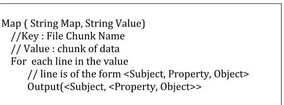
The Job Tracker assigns each of the Map functions with a chunk of the dataset,

where each tuple in the dataset is of the form <Subject, Property, Object>. The

pseudo code below shows the implementation of the Map function. The Map

function reads every tuple and generates the <key, value> pairs as an output,

where the value is a map of the predicate and the object corresponding to the

subject. Hence the Map function returns a list of <Subject, <Predicate, Object>

> pairs.

(54)

Map ( String Map, String Value) //Key : File Chunk Name // Value : chunk of data For each line in the value

// line is of the form <Subject, Property, Object> Output(<Subject, <Property, Object>>

Figure 5: Pseudo code for Map Function

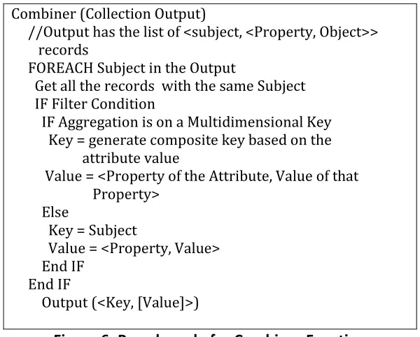
The Combine function is a sub-routine that is implemented within the Map

function and combines the related results of the Map. This function is executed

by the framework after the executing of the Map functions. All the values having

the same key are grouped together into a collection. If the user defined query

has any filter conditions defined on the dataset, then the corresponding <key,

Collection of values> are filtered out in this function. The pseudo code for the

(55)

Combiner (Collection Output)

//Output has the list of <subject, <Property, Object>> records

FOREACH Subject in the Output

Get all the records with the same Subject IF Filter Condition

IF Aggregation is on a Multidimensional Key

Key = generate composite key based on the attribute value

Value = <Property of the Attribute, Value of that Property>

Else

Key = Subject

Value = <Property, Value> End IF

End IF

Output (<Key, [Value]>)

Figure 6: Pseudo code for Combiner Function

In [9] the authors show that the tuples for which the filter condition is not true

will never be considered by the MD-Join and hence these tuples can be eliminated from the dataset. Thus MD (B,R,l,Θ), where Θ involves the attributes

of R is equivalent to MD(B, Selection on Θ (R), l, Θ); By eliminating the data

records for which the filter condition is not true, we are reducing the number of

records to be processed in the reduce function, thus increasing the efficiency.

3.2 Reduce Function Design

Set of keys and the collection of values are the input to the reduce function.

(56)

tuples. Base tuples are of the form <key, <BASE, NULL>>, where “BASE” is

used as a flag to perform the join operation. The fact tuples are of the form < key, [<property, value>]. For examples,

Example 3.2.1: To compute the number of each product purchased. The base tuples for this example will be of the type:

<PROD123, <BASE, NULL>> <PROD342, <BASE, NULL>> <PROD566, >BASE, NULL>> …

Consider the following to be the set of fact tuples containing the product id and the product purchase information.

(57)

All the properties and the corresponding values for the keys are collected

together. The algorithm for computing the aggregation is shown below. When a

match is found between the base and the fact tuple, the aggregation operation

is computed and the base tuple is updated with the value computed. Figure 7

shows the pseudo code for the reducer function.

Reduce(String Key, Iterator Value)

// The MD-Join Algorithm is implemented in this function FOREACH occurrence of the user defined condition in the fact set

IF Fact.key == Base.key

compute the Aggregation Function

And update the Base dataset, by replacing the NULL value in it.

Figure 7: Pseudo code for Reducer Function

Executing the Reduce function on the data shown in Example 2.3.1, we obtain

the following:

<PROD123, <LOC, NC>> <PROD123, <BASE, NULL>> <PROD342, <LOC, NY>> <PROD342, <BASE, NULL>> <PROD566, <LOC, NC>> <PROD566, >BASE, NULL>> <PROD934, <LOC, NC>> ..

(58)

The example above shows the execution of the reduce function on the

dataset, and how the aggregation values are updated on the Base

dataset.

As discussed in section 2.1, MD-join is designed to separate the tight coupling between the grouping attributes and the aggregation functions. Due to this

decoupling it is possible perform the grouping operation and the aggregation in

different functions. Since the grouping and the aggregation operations are

independent of each other, we can perform the grouping and the aggregation

operations in the Map and the Reduce functions respectively. Further, in

section 3.3, we show how the MD-join operator can be executed in parallel.

3.3 MD-Join - Intra-Operator Parallelism

In section 2.1 we discussed MD-Join for the sequential execution of the data. In this section, we will see how the MD-Join operator is amenable to parallelism by leveraging the results given in [9] which state the following:

Observation 3.3.1: If B and R are relations, B1, B2,....,Bm a partition of B,

l is a list of aggregate functions over columns of R and Θ is a set of

(59)

MD(B,R, l , Θ) = MD(B1,R, l , Θ)  MD(B2,R, l , Θ)  ...  MD(Bm,R, l ,

Θ)

This observation states that the query using MD-JOIN can be parallelized by dividing the base dataset across the processors and executing the MD-Join algorithm on each of them in parallel. This reduces the execution time for

processing the complex queries, but each processor still needs to have the

entire fact data set and iterate through it completely to check if there is a

matching key found for computing aggregation.

Based on the above conclusion the following observations were made,

Observation 3.3.2: In MD(B,R,l,Θ), B can be partitioned into B1 

B2…  Bn where Bi = σi(B), where σi is a range selection based on the

attributes on B. Similarly R can be partitioned into R1  R2…  Rn

where Ri = σi(R), where σi is a range selection based on the

attributes on R. The same selection function is used for both base and the fact table partitioning in such a way that the same range of selection is performed. Hence,

(60)

This observation states that the query using MD-JOIN can be parallelized by dividing both the base dataset and the fact dataset across the processors such

that every processor gets the same range of base and fact data. Thus the MD

-Join algorithm can be executed on each of them in parallel for the subset of the fact and the base data.

This section shows how the MD-join operator can be implemented as a

map-reduce function. Since this is a low level implementation of the operator, any

customized computation that needs to be done, requires the user to change the

Map and the Reduce functions. As discussed in section 2.2, the user

customized code does not allow the efficient optimization. In the next section

we provide a set of new operators for Pig Latin language to perform complex

(61)

Chapter 4 Extending Pig Latin for analytical processing of RDF

Pig Latin provides various operators like the JOIN, FILTER, GROUP and

COGROUP which can be used to support the basic analytical queries. Example 4.1: Consider the data shown in Table 2 to get all the list of all

the customers who bought products in location NC, we need to execute

the following queries in Pig Latin

Raw_data = LOAD “sales.rdf” as (Subject, Predicate ,Object);

Join_res = Join Raw_data by Object, Raw_data by Subject

Res = FILTER Join_res By $1 eq “Bought” AND $4 = “location” AND $5 =

(62)

Output = FOREACH Res GENERATE ($0, $1, $5);

In Example 4.1 we perform LOAD, JOIN, FILTER and FOREACH operations.

Each of these operations requires reading the data file once completely. Thus

the above query collectively reads the data file five times resulting in cost

inefficient query execution. Further, the complex queries require executing

multiple group operations with the different aggregation functions resulting in

more expensive query executions.

One alternative is to implement the complex data processing using the UDF

that allows the users to implement the desired functionality as a user defined

function. However, in our earlier discussions we have mentioned the

disadvantages of this approach. This section presents an extension to the Pig

Latin language that includes the specialized functions that allow the complex

data processing tasks to be specified in terms of the MD-join operator. Also, the additional classes of expressions are introduced in the language to deal with

the graph structured nature of the RDF data.

In the following sub sections, we define the three functions that can be used in

(63)

Class expressions or the Property expressions. Class expressions are

represented by type : class_name, and are used to specify the class of the subject in the qualifying triple. For example, the expression “type:Customer”

specifies that the qualifying tuple‟s subject will be of the type Customer. The

properties are represented similarly using the property expressions. The graph

based nature of the RDF data makes it necessary to specify the navigational

patterns of a set of the desired objects that can be represented using property

expressions. For instance, the path expression to represent the navigation from

the Customer C1 to the product P1’s price can be represented as “bought.price”. These kinds of expressions represent the relation between the

tuples and are hence useful to in performing the JOIN operation between the related tuples.

4.1 Generating Fact Dataset: GFD

MD-join operation requires a fact dataset and a base dataset to execute the algorithm. In order to generate the fact dataset, we need to load the RDF file

initially. As mentioned earlier, the format of an RDF file is of the form <Subject,

Property, Object>, which differs from the format of the relational data (sequence

(64)

input file and must be handled during the load process. Thus we call the LOAD operator of Pig Latin along with the GFD operator. To generate the fact dataset from an RDF file “input.rdf”, a specialized class for GFD needs to be added to the Pig Latin library. The following shows the syntax of the GFD function:

fact_dataset = LOAD 'input.rdf' USING

GFD(Class_Expression; property_expressions;

aggregation_pathexpression; filter_pathexpression’);

In this syntax, input_dataset is the data loaded from the RDF file. Class_Expression indicates the value of the subject in the input_dataset.

property_expressions indicates the properties for which the aggregation needs to

be computed. The filter_pathexpression indicates the properties for which the filter conditions needs to be checked. Finally, the aggregation_pathexpression holds the property on which the aggregation operation is performed. The LOAD operator reads each line from the input.rdf file and calls the GFD operator. The

(65)

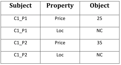
necessary JOIN operations are preformed to reassemble the tuples. Generating the Fact tuples for the example 4.1 is as shown below. Figure 8 shows the steps

in executing GFD for the example given.

fact_dataset = LOAD 'input.rdf' USING

GFD(TYPE:CUSTOMER; BOUGHT.LOC,BOUGHT.PRICE;

BOUGHT.PRICE; BOUGHT.LOC’);

<c1, type, Customer> <c1, bought, P1> <P1, loc , NC> <P1, price, 25>

<c1,< type, Customer>>

<c1, <bought, P1>>  <P1, <loc , NC>> <P1, <price, 25>>

<C1_P1 , Price 25 > <c1_P1, Loc, NC> LOAD

GROUPBY

JOIN

(66)

GFD performs the required join operations on the related tuples and generates result of the form <Subject, Property, Object>. The subset of the output for the

above query is of the form:

Table 10: Shows the result obtained after executing GFD

Subject

Property

Object

C1_P1 Price 25

C1_P1 Loc NC

C1_P2 Price 35

C1_P2 Loc NC

The result generated using this operator is called as the fact dataset. Fact dataset is a subset of the tuples that are required to compute the result for the

user given query. Within the GFD function, we call the STORE function to store this fact dataset in an intermediate file called the MDJ.rdf. The data from the file

is later used by the MDJ operator while performing the MD-join operation, which is discussed in section 4.3.

4.2 Generating Base Dataset: GBD

Section 2.1 describes a simple algorithm for a MD-Join operator. The algorithm

(67)

which the aggregation needs to be computed. For every tuple in the fact

dataset, the corresponding combination in the base dataset is obtained and the

aggregation results are updated in the container tuples. Similar to the GFD, the

GBD operator is executed along with the LOAD function. base_dataset = LOAD 'input.rdf' USING

GBD(Class_Expression; property_expressions; FLAG’);

As in GFD, the class_expression and the property_expression are path expression to indicate the relationship that exists between the tuples having the

same subjects. The Flag holds either the value “NULL” or “BOTH” that indicates

that the key for the Aggregation is either the properties got from the

property_expressions or a combination of the property value and the type class.

The tuples generated by the GBD are of the type <Subject, Base, NULL> where “Base” is a flag that indicates that the tuple belongs to the base dataset. The

NULL value will be replaced by the value computed by the aggregation function

when executing MDJ operation. Generating the Fact tuples for the example 4.1 is as shown below. Figure 9 shows the steps in executing GFD for the example

given.

(68)

(TYPE:CUSTOMER; BOUGHT.LOC,BOUGHT.PRICE; NULL);

The result generated after the execution of GBD is shown in the Table 4

Table 11 : Subset of the result generated after the GBD operation

Subject Property Object

C1 BASE NULL

C2 BASE NULL

<c1, type, Customer> <c1, bought, P1> <P1, loc , NC> <P1, price, 25>

<c1,< type, Customer>>

<c1, <bought, P1>>  <P1, <loc , NC>> <P1, <price, 25>>

<C1 , BASE, NULL > LOAD

GROUPBY

JOIN

(69)

The tuples generated by the GBD operator are referred to as the base tuples. Base tuples are initialized with a NULL, for each object corresponding to the

subject. The NULL values are updated during the aggregation operation.

Within the GBD function, we call the STORE function to append the base dataset into the same MDJ.rdf file. This file is later loaded by the MDJ operator while performing the JOIN operation and is discussed in the next section.

4.3 Multi-Dimensional Join: MDJ

After the generation of the base tuple and the fact tuple sets, the next step is

the execution of the MD-Join algorithm on these datasets. In order to perform the multi dimensional JOIN operations in the Pig Latin, the MDJ operator class is included as a part of the language library. The MDJ operator executes on the data present in the “MDJ.rdf” file created by the GFD and GBD operators as mentioned in section 4.1 and 4.2. This operator takes as input the filter

condition on which the aggregation needs to be computed and the aggregation

function such as the SUM, COUNT, MAX, MIN, AVG. The syntax for the MDJ operator is as follows: