ABSTRACT
HAN, ZHEN. Statistical Methods for Relational Data: Visualization, Classification, and Topic Modeling on Networks. (Under the direction of Alyson Wilson.)
Data structured in a relational format, also called networks, are ubiquitous in various areas of science. The rapid growth of the internet, along with the popularity of online social networks, have fueled huge interest in network modeling. Specifically, statistical models for network analysis have evolved to be a very important tool in various areas; for example, network visualization [29], link prediction [15], community detection [24], and node classification [51].
In Chapter 2, we focus on dimension reduction and visualization in networks and propose a parallelized procedure for network visualization using a latent space model. Latent space models provide an interpretable spatial representation of social relationships. However, model estimation is slow for large networks. We describe how to fit a latent space model using a parallel gradient descent algorithm with momentum and learning rate adaptation. Our method effectively boosts the estimation speed for networks of a few thousand nodes by several orders of magnitude. We compare our methods with multiple graph visualization/dimension reduction methods and present results for a few examples using an implementation on Graphical Processing Units (GPUs). We also discuss how to extend these results to larger networks and how to handle sparsity.
©Copyright 2016 by Zhen Han
Statistical Methods for Relational Data: Visualization, Classification, and Topic Modeling on Networks
by Zhen Han
A dissertation submitted to the Graduate Faculty of North Carolina State University
in partial fulfillment of the requirements for the Degree of
Doctor of Philosophy
Statistics
Raleigh, North Carolina
2016
APPROVED BY:
Brian Reich Hua Zhou
Nagiza Samatova Alyson Wilson
DEDICATION
BIOGRAPHY
ACKNOWLEDGEMENTS
First of all, I would like to express my utmost gratitude to my advisor Dr. Alyson Wilson for her continued support and mentoring throughout my study here at NC State. It has been a highly rewarding experience working with her.
I would like to take this opportunity to thank my committee members, Dr. Nagiza Samatova, Dr. Brian Reich, and Dr. Hua Zhou for their constructive comments and suggestions for this thesis.
I would also like to thank MaxPoint for their generous funding and offering me the opportunity to gain valuable hands-on experience in the data science industry.
TABLE OF CONTENTS
List of Tables . . . vii
List of Figures . . . viii
Chapter 1 Introduction and Motivation . . . 1
1.1 Background and Notation . . . 1
1.2 Visualization and Dimension Reduction . . . 2
1.3 Node Classification . . . 4
1.4 Relational Topic Modeling . . . 5
1.5 Contributions and Outline . . . 6
Chapter 2 Fast Network Visualization and Dimension Reduction . . . . 8
2.1 Overview . . . 8
2.2 Background and Related Works . . . 9
2.3 Model Description and Estimation . . . 12
2.4 Simulation Study . . . 17
2.5 Examples . . . 22
2.6 Modeling Sparsity . . . 26
2.6.1 NCAA Example Revisited . . . 29
2.7 Discussion . . . 31
Chapter 3 Node Classification on Networks. . . 32
3.1 Literature Review . . . 32
3.2 Background and Motivation . . . 35
3.3 Dynamic Stacking Model . . . 38
3.3.1 Notation for the Stacked Generalization Model . . . 38
3.3.2 Generalized Varying Coefficient Model through Smoothing Splines 40 3.4 Simulation Study . . . 44
3.5 Examples . . . 46
3.6 Discussion . . . 48
Chapter 4 Topic Modeling on Networks . . . 52
4.1 Literature Review . . . 52
4.2 Background and Related Work . . . 54
4.3 Generalized User Interests Model . . . 56
4.3.1 Modeling Documents . . . 56
4.3.2 Modeling Edges . . . 58
4.4 Inference and Parameter Estimation . . . 61
4.4.2 Parameter Estimation . . . 65
4.5 Model Comparison . . . 66
4.5.1 Simple Demonstration . . . 66
4.5.2 Simulation Study . . . 66
4.6 Analysis of NSF Awards . . . 68
4.7 Discussion . . . 75
Chapter 5 Concluding Remarks and Future Work. . . 77
LIST OF TABLES
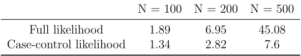
Table 2.1 CPU time of case-control likelihood and full likelihood, for different network sizes with average degree 10. All times are in seconds per
1000 likelihood evaluations. . . 21
Table 2.2 GPU computation time for the latent space model for different net-work sizes with average degree 10. The times are measured in sec-onds per 1,000 parameter updates. The GPU used is NVIDIA Tesla M2070-Q GPU with 5.3GB available RAM. . . 21
Table 2.3 Accuracy comparison across different embedding methods . . . 30
Table 3.1 AUC score comparison between the proposed method and bench-marks. For level-1 generalizers, methods1 use z+ 1i and z + 2i as covari-ates, methods2 containsu i as an extra feature, and methods3 further include linear interaction termsuiz1+i, anduiz2+i. The standard devi-ation of the accuracy score is calculated from 50 repetitions and is shown in parenthesis. . . 46
Table 4.1 Method comparison of estimating β . . . 69
Table 4.2 Sample entry in NSF award query . . . 70
Table 4.3 Frequency table for the number of abstracts for a node . . . 72
Table 4.4 Frequency table for the number of nodes for an unique abstract . . 72
Table 4.5 RUI Model . . . 73
Table 4.6 RTM Model . . . 73
Table 4.7 RUI in a polluted dataset . . . 74
LIST OF FIGURES
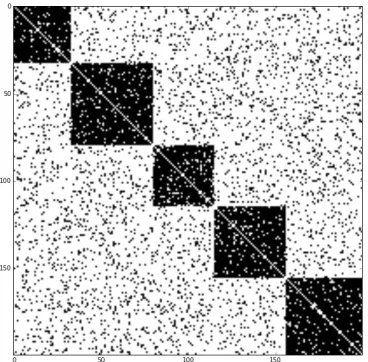
Figure 2.1 Adjacency matrix of the simulated network . . . 17
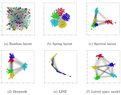
Figure 2.2 Visualize the simulated network with different graph layout algo-rithms . . . 18
Figure 2.3 Visualize the NCAA network . . . 23
Figure 2.4 Visualize the Blog network . . . 24
Figure 2.5 Visualize the karate network . . . 25
Figure 2.6 Visualize the Book network . . . 26
Figure 2.7 Histogram of log(neighbor count) . . . 28
Figure 2.8 NCAA network revisit with a sparse approach . . . 30
Figure 3.3 Classification accuracy differences between the proposed method and multiple standard level-1 generalizers for 1000 experiments. The vertical dashed line means zero difference. In (a), the proposed method outperforms Lasso regression 92% of the time. In (b), the proposed method outperforms Ridge regression 91% of the time. In (c), the proposed method outperforms Logistic regression 87% of the time. By assuming the normality of the classification accuracy difference distribution, it can be shown that our proposed model significantly outperforms all the benchmarks at p-value <0.01. In (d), one set of fitted coefficient curves is shown. . . 50
Figure 3.4 For each of the 1000 repetitions, we calculate the difference in the number of correctly classified nodes at different closeness centrality levels between the dynamic stacking model and benchmarks. In (a) – (c), we calculate the group mean and a 95% confidence interval. (d) shows a density distribution of the closeness centrality for all nodes in the graph. . . 51
Figure 4.1 A graphical model for a two-user segment of the full RUI model. The graph denotes the conditional dependence structure in the model, where nodes are variables and plates are repeated sub-units. In the RUI model, the edge values are dependent on the topic as-signments for every document consumed by each user, with global dependency parametersη and v. . . 59
Figure 4.2 β estimation comparison: graph (A) shows the true β, graph (B) shows the estimated ˆβ without replicated documents, and graph (C) shows the estimated ˆβ with a random document replicated 100 times. . . 67
Chapter 1
Introduction and Motivation
Data structured in a relational format, also called networks, are pervasive across many areas of science. For example, a network can represent different molecules and their interactions, or analyze protein interaction and identify protein groups. It can be used to model a power grid, analyze an online social network, or identify malicious websites based on internet traffic. The rapid growth of the internet, along with the popularity of online social networks, have sparked huge interest in network modeling. Specifically, statistical models for network analysis have evolved to be an important tool in various areas; for example, network visualization, link prediction, community detection, node classification, and topic modeling.
1.1
Background and Notation
A network can be categorized into a directed network or an undirected network. In a directed network, E is non-symmetric, meaning (νi, νj)∈ E does not imply (νj, νi)∈ E. In contrast, E is symmetric for a undirectednetwork. For example, on LinkedIn.com, professionals are connected by business relationships. When two individuals establish a connection, each one will be in the other person’s contact list. The relationship here is non-directional. However, onTwitter.com, people are connected by their social interests. A person can follow the updates of another person, but this does not imply the other person will follow back. The relationship here is directional.
Often the inter-relationship in V is more than a dichotomous relationship. In a weighted network, we may observe a weight associated with each edge in E. For ex-ample, in a co-authorship network, an edge represents the number of papers published by two authors, or in a transportation network, an edge can represent the traffic flow between destinations. In contrast, in a unweighted network, edges have a binary rela-tionship with constant weight equal to 1.
Usually, a network can be represented by a square matrix Y of size N × N, also called an adjacency matrixor sociomatrix. For an undirected unweighted network, Y is a symmetric matrix with binary entries of value 0 or 1. Here Y encodes the presence or absence of connections between all pairs of nodes on the network. For a directed unweighted network, Y is not symmetric. For weighted networks, the elements in Y can encode the weights of edges between a pair of nodes.
1.2
Visualization and Dimension Reduction
underlying interaction patterns and the community structure within a network. Many visualization methods are available for relational data. Force-directed graph layouts are a popular set of visualization algorithms widely implemented in commercial software. Inspired by physics principles, they position nodes by minimizing overall system energy [5].
Network data are presented in a relational format that is not directly analyzable by most statistical models. As a result, dimension reduction becomes a valuable tool. It extracts a fixed length feature vector for each node by encoding the underlying network relationship. Network visualization methods are a special class of network dimension re-duction techniques where we set the length of the feature vector to be 2 (for a 2-D plot) or 3 (for a 3-D plot). For network dimension reduction, the latent space model [30, 53] assumes that each node has an unknown position in aK-dimensional latent space, which is characterized by an Euclidean space. The relative position of two nodes in latent space determines the edge probability in the observed network. The optimal positioning is learned by Maximum Likelihood Estimation (MLE). In the computer science literature, a recently published algorithm, DeepWalk [50], learns a K-dimensional latent represen-tation of a network by initiating truncated random walks at each node and collecting the path information. LINE [56] considers a specially designed objective function that incorporates both the local (first order) and global network structures (second order) and then optimizes the objective function to achieve network dimension reduction. The well-studied spectral methods work directly by decomposing the graph Laplacian matrix and use the top K eigenvectors as a latent representation for the network. The graph Laplacian can be written as:
where D is a diagonal matrix of sizeN ×N with Dii equal to the degree of node νi. After projecting nodes onto a K dimensional space, many statistical models and machine learning algorithm with fixed length features are applicable. Dimension reduction has been an important bridge connecting network data and traditional statistical and machine learning models. In Chapter 2, we focus on a GPU-accelerated method based on the latent space model for network visualization and dimension reduction. Our method experiments with the massively parallel structure of Graphical Processing Units (GPUs) and achieves several order of magnitude speedup compared with benchmarks.
1.3
Node Classification
In many situations, we may observe rich node features on a subset of V. For example, in a citation network, where two academic papers are connected if one cites another, aside the network relations, we may observe abstracts, key words, and journal for a subset of papers. For another example, in a social network, where edges represent friendship, we may have the genders, ages, income levels, and descriptions of some self-disclosing users in the network.
Many classification methods have been developed over recent years [49] that can bor-row strength from the labels and features of a node’s neighborhood for better prediction. However, there has been little effort into studying how to ensemble multiple node clas-sification methods to achieve lower clasclas-sification error overall on a network. In Chapter 3, we will focus on a dynamic stacking model that can dynamically employ a pool of heterogeneous classifiers to achieve significantly lower classification error rates for node classification on networks.
1.4
Relational Topic Modeling
For a pool of independent text documents, statistical models like Latent Dirichlet Al-location (LDA) [9] and its many variants [58, 31, 44] have been studied extensively across many applications, from recommendation systems to topic classification. When documents are inter-related through edges, the link structure provides another valuable source of information for uncovering and understanding the topic structure of individual documents.
Why would the link structure of a document network matter to understanding indi-vidual document topics? In a citation network where edges are randomly drawn between papers, the network structure would truly have no relationship with an individual paper’s content. However, in practice, when one paper cites another or “shares” an edge with another paper, chances are these two paper will have similar research topics.
open discussions, and connect with their colleagues. In such a network, instead of a single paper per node, as with a traditional citation network, one may observe multiple papers on one node. To make matters even more complicated, co-authors may post identical papers, which means the same paper may be owned by multiple nodes. Without careful handling of the duplicate papers, we are facing a data pollution problem [47], which could potentially bias our understanding of the overall topic structure in the corpus. In an effort to model networks with such text features, in Chapter 4, we develop a Relational User Interests (RUI) model for a user network with collections of text documents as node attributes. The proposed method can jointly model the network linkage structure and the topics of individual documents, and by combining both sources of information, it is able to discover topics that are more predictive of the network structure and make more accurate predictions based on individual text documents.
1.5
Contributions and Outline
Chapter 2
Fast Network Visualization and
Dimension Reduction
2.1
Overview
dimension reduction. All of these graph layout methods learn some representation of the network; however, in this chapter, we will illustrate that the distances in the layout are often not easily interpretable.
In many social networks like LinkedIn.com, the more characteristics shared by two individuals – like educational background or geographical location – the more likely these two individuals will establish a connection. Intuitively, if we observe a large number of connections within a tight group of nodes, a social “community,” it is likely that this group of nodes share similar characteristics. In other words, this group of nodes will likely have nearby locations in the characteristics space. Following this intuition, Hoff et al. [30] introduced the latent space approach to social network analysis. Although it can provide a easily interpretable spacial representation of a network, the model estimation is painfully slow. In this paper, we propose a slightly modified latent space model and to accelerate model fitting by using Graphical Processing Units (GPUs).
2.2
Background and Related Works
in the latent space.
log odds(yi,j = 1|zi,zj,xi,j, α,β) =α+βTxi,j− |zi−zj|, (2.1)
wherexi,j is the observed feature vector of the edge between nodei andj,zi and zj are latent position vectors in R2, | · |is the l
1 norm of a vector, α is the intercept term, and
β is coefficient vector. By assuming the links are independent conditional on the latent space, the log-likelihood function can be written as a function of Z, α, and β, where
ZT = [z1,· · · ,zN]:
L(Z, α,β) =
X
i6=j
logp(yi,j|Z, α,β). (2.2)
In [30], a Bayesian approach was proposed for estimating the latent space model by using diffuse independent normal priors forα,β, andZ. However, the diffuse independent normal priors forZ may not accurately capture our prior knowledge about the clustering structure of social networks in the latent space. In [26], a generalized latent space model was proposed for clustering analysis by assuming thatZfollows a mixture of multivariate normal prior distribution:
zi iid ∼
G X
g=1
λgMVNk(µg, σg2Ik), (2.3)
where G is the number of clusters, µg and σg2 are the multivariate normal distribution parameters for the gth cluster, and λg is the probability of node i coming from the gth cluster. As described in [30], the estimation and inference for the latent space model are performed in two steps:
maximum likelihood estimate (MLE) ˆZ of Z.
2. Run a Markov Chain Monte Carlo (MCMC) algorithm starting at ˆZ to draw sam-ples from the posterior distribution of the latent positions, Z, and model parame-ters, α and β.
The log-likelihood function in equation (2.2) is not concave in terms of {Z, α,β}. Direct optimization of the log-likelihood function is subject to the choice of starting values and may get stuck in local optima. As a remedy, one may first construct a set of dissimilarities based on the geodesic distances between nodes and then apply multidimensional scaling methods to get an initial estimateZ0, which can serve as the starting point for a nonlinear optimization routine.
With the estimated ˆZ, the MCMC algorithm constructs the posterior distribution of the latent positions, which in turn summarizes the uncertainty in the estimated ˆZ. However, every MCMC step involves the calculation of the complete likelihood function, with O(N2) complexity. This makes the latent space model computationally infeasible for networks with more than 1,000 nodes [53]. To achieve fast calculation of the likelihood function, an approximation method was proposed in [53]. It approximates the complete likelihood function by constructing an unbiased estimator using a small set of connected and non-connected edges. This method was adopted from case-control studies in epidemi-ology, where the connected edges are cases and non-connected edges are controls. By not iterating every possible pair of nodes on the graph, the algorithm manages reduces com-plexity to O(N). Overall, latent space models can provide an intuitive and interpretable model-based visual representation of relational data.
a shrinkage term. We focus on directly optimizing the objective function using first-order optimization methods to get point estimates for the MLE ˆZ. We speed up the computation by utilizing the massively parallel structure of GPUs, and we are able to achieve several orders of magnitude of improved computational efficiency as compared to CPU implementations. We also discuss how to address the sparsity observed in many large networks and scale our method effectively.
2.3
Model Description and Estimation
Ignoring the covariates associated with edges, we model the probability of forming a connection between two nodes, i and j, as follows:
pij = Prob(yij = 1) =f(α+β|zi−zj|22), (2.4)
where f(·) is the logistic transformation:
f(x) = 1
1 + exp(−x) . (2.5)
ziis the unobserved position of nodeiin the latent space, and it needs to be estimated.β is a scale parameter that controls the tightness of the latent space, andα is the intercept term. The probability function f(x) is a smooth monotone decreasing function bounded between (0,1] with
Assuming the edges are independent conditional on the latent positions of nodes, we can write the log-likelihood function as:
L(z1,· · ·,zN, α, β) = X
i6=j
{yijlog(pij) + (1−yij) log(1−pij)}. (2.7)
Note that the log-likelihood is a function of each node’s positionz1,· · ·,zN in the latent space and model parameters α and β. To insure the identifiability of β and the proper centering of z1,· · · ,zN, we add a regularization term to the objective function:
O=−L+λ
N X
i=1
|zi|22. (2.8)
λcontrols the “radius” of the graph, where a largeλ shrinks the scale of the latent space. However, the model is not sensitive to the exact value of λ, as a large λ value can be offset by a largeβ. We will discuss its interpretation shortly.
Next, we derive the first order gradients of the objective function with respect to
z1,· · · ,zN, α, β. Denote f(α+β|zi−zj|2) by pi,j. Then we have:
∂O ∂zik
=− X
j∈connected nodes
2β(1−pi,j)(zik−zjk) (2.9)
+ X
j∈non-connected nodes
2βpi,j(zik−zjk)
+ 2λzik ,
toward origin with strength controlled byλ. The gradients ofα, β are:
∂O
∂α =−
X
iconnected toj
(1−pi,j) (2.10)
+ X
inot connected toj
pi,j ,
∂O
∂β =−
X
iconnected toj
(1−pi,j)|zi−zj|22 (2.11)
+ X
inot connected toj
pi,j|zi−zj|22 ,
where i, j = 1,· · · , N, i 6= j, and k = 1,· · · , K. K is the number of dimensions of the latent space.
For model estimation, we directly minimize the objective function in equation (2.8) using the gradient descent algorithm to find an estimate for ˆZ. To speed up model training, we further add momentum and learning rate adaptation into the optimization routine. The gradient descent algorithm, also known as steepest descent, is one of the simplest and most popular algorithms in machine learning. It starts with an initial guess, {Z0, α0,β0}and then iteratively updates parameters using a step size s, in the direction
At the t-th iteration, the update for Z as:
Zt+1 =Zt−st∇Ot+m4Vt (2.12)
4Vt =Zt−Zt−1, (2.13)
wherest is the learning rate, which decays witht,m is the momentum term, and4Vtis the velocity at iterationt. Intuitively, at each iteration, we updateZ in a direction that combines the negative gradient of the objective function and the previous update. The update schemes for α and β follow a similar structure with potentially different st and
m. As one can see in equation (2.9), at a specific iteration, the gradient computation and parameter updates for {zik, i = 1,· · · , N and k = 1,· · · , K, α, β} are all independent. One can naturally accelerate the training by parallelizing the gradient calculation and parameter updates.
for updating Z is shown in Algorithm 1. The updates on α and β can be done trivially, and they are left out in the presentation of the algorithm for clarity.
Algorithm 1 Gradient Descent Algorithm using GPU
1: Initialize starting values for Z0, α0, β0, and copy to the device memory on GPU.
2: repeat
3: Initialize N threads on GPU, and for thread i • Calculate the gradients for zi1,· · · ,ziK.
• Determine the new values, z∗i1,· · · ,z∗iK.
4: Execute N threads and wait for completion.
5: Synchronize across the whole GPU and make updates on the model parameters {Z, α, β}.
6: untilChange in the objective function value falls below some pre-specified threshold or a maximum number of iterations is reached.
The model discussed in this chapter differs from the original latent space model in a few aspects:
• We use the square of the L2 norm to measure the distance on the latent space.
• We add a scale parameter and a shrinkage term to gain flexibility and stability in
the model training.
• We work on the direct optimization of the modified likelihood function and
Figure 2.1: Adjacency matrix of the simulated network
2.4
Simulation Study
We examine the proposed method using simulated data generated by a stochastic block model (SBM) [23]. In SBMs, nodes are partitioned into M non-overlapping communities
C1,· · ·,CM. The inter-community edge probabilities are specified by a symmetricM×M matrix, P, such that for two nodes u ∈ Ci, v ∈ Cj, the probability of establishing an edge is Pi,j. Following this model, a random network, G≡ (V,E), can be simulated by the following generative process:
1. Assign each node to one of theM communities,C1,· · · ,CM, with equal probability.
2. For each pair of nodes (νi, νj)∈ V ⊗ V:
• Suppose the community labels forνi, νj are ci, cj.
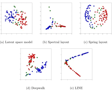
(a) Random layout (b) Spring layout (c) Spectral layout
(d) Deepwalk (e) LINE (f) Latent space model
Figure 2.2: Visualize the simulated network with different graph layout algorithms
nodes using the eigenvectors of the graph Laplacian. The spring layout in Figure 2.2b places nodes using Fruchterman-Reingold force-directed algorithm [20]. A force-directed algorithm considers the graph as a system of electrically charged balls (nodes) and con-necting springs (edges). Nodes are mutually repulsive, but the springs between connected nodes pull the two together. The final layout of the force-directed algorithm minimizes the “energy” of the system. For Deepwalk, we use the implementation provided by [50] with dimension equal to 2. For LINE, we use the implementation provided by [56] with dimension equal to 2. For the latent space model, we use the spectral layout as the starting point for the optimization routine and run for 1000 iterations.
a roughly symmetric display where nodes from the same community are placed near the same position. In addition, the distances in the visualization between nodes and commu-nities is statistically tied to their connection probability. Therefore, our model provides a more intuitive and comprehensive visual representation of the network.
Next we test the computational performance of the GPU-accelerated implementation against the original latent space model [30] and the fast-inference latent space model us-ing the case-control approximate likelihood [53]. The original latent space model makes inference through an iterative MCMC process. In each step, it requires evaluation of the complete likelihood function, with complexity O(N2). This likelihood evaluation is the bottleneck for the latent space model in its application to large networks. The fast-inference latent space model approximates the full likelihood by constructing an unbiased estimator using a small subset of allN2 possible node pairs. Instead of iterating through all node pairs on the graph, the fast-inference algorithm only focuses on node pairs that fall within a certain distance. This distance is measured by the shortest path between two nodes [53]. As a result, it does not need to consider every pair of nodes and can greatly boost the computation speed for the likelihood evaluation, given that we have the dis-tance metrics for each pair of nodes in the network. However, it is not computationally free to obtain the shortest path distance between every pair of nodes in the network, also known as the All Pairs Shortest Paths problem (APSP). The Floyd-Warshall algorithm finds shortest paths in a weighted graph with positive or negative edge weights with a computation complexity O(N3) [19]. For unweighted undirected graphs, the best com-putation complexity so far is O(N E) , where N is the number of nodes and E is the number of edges for a sparse network (E N1.376) [13].
simulated networks of various sizes. We show the computational performance comparison table from [53] in Table 2.1 and present the performance of our GPU-accelerated method in Table 2.2 using networks of the same sizes so they are comparable. The computation time of our method increases linearly when the network size is below some threshold, which is dependent on the specific GPU used. When N = 500, we have achieved more than 16 times better performance compared with the original CPU-based latent space model, and about 3 times better performance compared with the approximate method with case-control likelihood.
Table 2.1: CPU time of case-control likelihood and full likelihood, for different network sizes with average degree 10. All times are in seconds per 1000 likelihood evaluations.
N = 100 N = 200 N = 500 Full likelihood 1.89 6.95 45.08 Case-control likelihood 1.34 2.82 7.6
Table 2.2: GPU computation time for the latent space model for different network sizes with average degree 10. The times are measured in seconds per 1,000 parameter updates. The GPU used is NVIDIA Tesla M2070-Q GPU with 5.3GB available RAM.
N = 100 N = 200 N = 500 Full likelihood 0.53 0.93 2.70
N =1000 N = 2000 N = 4000 Full likelihood 5.11 9.86 19.42
of the computation time with the number of nodes in the graph as shown in Table 2.2. This is because we can allocate the N2 computational load to N computation threads when N ≤ NMax. NMax is the maximum number of concurrent threads that can run in parallel on GPU given that particular GPU hardware, current memory consumption, and implementations. For the particular setting in the discussion above,NMaxis around 7000, after which the computation time increases quadratically.
2.5
Examples
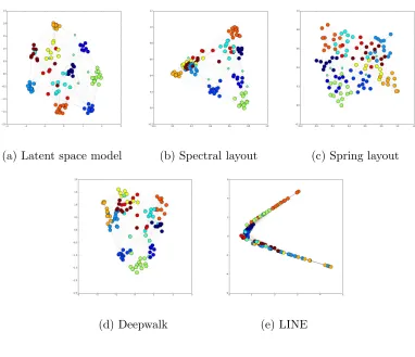
We analyze four well-known network datasets using the proposed method. These datasets are attractive because we have the ground-truth labels for visually assessing performance. Figure 2.3 presents the network of 2001 National Collegiate Athletic Association (NCAA) American football games between Division I-A colleges [41]. In this network, there are 115 nodes and 615 edges, where nodes represent college teams and edges repre-sent whether these two teams played against each other during the regular season. Most colleges in Division I-A are grouped into athletic conferences. Teams within a conference play against each other more often than with outside teams. We run our model with the starting point chosen by the spectral layout and run for 1000 iterations. The results are shown in Figure 2.3. Colors represent ground truth conferences partitions. One can clearly see that our visualization method reflects the underlying structure in the network.
hy-(a) Latent space model (b) Spectral layout (c) Spring layout
(d) Deepwalk (e) LINE
Figure 2.3: Visualize the NCAA network
perlinks between blogs. These blogs are divided into two groups: liberal and conservative. We run our model with the starting point chosen by the spectral layout and run for 1000 iterations. The results are shown in Figure 2.4, where the colors represent the ground truth groups in the network. One can see that our visualization method clearly reflects the underlying structure in the network.
(a) Latent space model (b) Spectral layout (c) Spring layout
(d) Deepwalk (e) LINE
Figure 2.4: Visualize the Blog network
of members were present in the network: one affiliated with the club instructor and one affiliated with the club administrator. We run our model with the starting point chosen by the spectral layout and run for 1000 iterations. The results are shown in Figure 2.5, where the colors represent the ground truth groups in the network. One can clearly see that our visualization method reflects the underlying structure in the network.
(a) Latent space model (b) Spectral layout (c) Spring layout
(d) Deepwalk (e) LINE
Figure 2.5: Visualize the karate network
These books are naturally divided into three groups: liberal, neutral, and conservative. We run our model with the starting point chosen by the spectral layout and run for 1000 iterations. The final visualization is presented in Figure 2.6, where colors represent the ground truth groups in the network. One can clearly see that our visualization method reflects the underlying structure in the network.
(a) Latent space model (b) Spectral layout (c) Spring layout
(d) Deepwalk (e) LINE
Figure 2.6: Visualize the Book network
2.6
Modeling Sparsity
complexity.
As discussed in [4, 15], in many real-life examples, adjacency matrices with binary entries are often highly sparse. For example, on LinkedIn.com, nodes represent people, communities represent social groups, and edges identify connections among people. A large portion of the non-connections on the network are because of the limited opportu-nities for contact between people. These non-connections should properly be treated as missing and be left out of the likelihood [30]. In this section, we propose a modification of our algorithm that accounts for the missing observations, which enables it to scale to massive networks and handle the sparsity problem effectively.
The small-world phenomenon, also known as six degrees of separation, has been dis-cussed widely [60]. The small world theory says that everyone in the world is six or fewer steps away, and through a chain of friends’ introductions, any two people can have a chance to meet in a maximum of six steps. However, you haven’t met everyone on the planet; when someone is many connections away from you, you may not be even aware of his existence. This is the way we distinguish between missing connections and ob-served non-connections in our algorithm. The rule is to treat people that are more than
S connections away from a node as missing observations. With a large enoughS, we can recover our previous algorithm for dense networks.
For small S, our algorithm runs much faster for real-world networks where we have millions of nodes, edges, and missing observations. By taking account of the sparsity, the algorithm only has to iterate through a small-neighborhood subset of the network for each node. Even though the running time complexity for the worst-case scenario (a fully connected network) is stillO(N2), we gain several orders of magnitude speed-up for sparse networks, as demonstrated in the following example.
presents a co-authorship network, where two authors are connected if they publish at least one paper together. The ground truth community is identified by publication venue, e.g., journal or conference, and authors who published in a certain journal or conference form a community. The data has 317,080 nodes and 1,049,866 undirected edges. The histogram for the number of neighbors with S = 2 is shown in Figure 2.7a, and the histogram for the number of neighbors with S = 3 is shown in Figure 2.7b.
(a)S= 2 (b)S= 3
Figure 2.7: Histogram of log(neighbor count)
Without accounting for sparsity, each node the algorithm needs to consider each of the other 317,080 nodes, and we have bias in the final estimated latent space, as we count the missing observation as observed. After removing the missing observations with a pre-specifiedS, we only need to iterate through a small set of nodes. This modification removes the bias from the sparse data and makes the computation several thousand times faster. For example, withS= 2, we only need to iterate throughe4 = 55 nodes on average instead of 317,080 nodes.
GPU. Take S = 2 as an example. From the neighbor count distribution in Figure 2.7a, some nodes are the hubs of the network and have many more neighbors within two connections. However, the majority of nodes have less than 100 neighbors. This poses a problem for computational load balancing. On the GPU, threads are organized into blocks. Within a block, if one thread has a lot of computation while other threads in the same block have little work to do, the whole block will be waiting for the last thread to finish before the GPU can reallocate its resources to a new block of threads. Therefore, ideally we want each thread to have an equal workload to achieve the most benefit from parallel computing. To achieve load balance, we can sort nodes based on their number of neighbors and assign nodes with similar numbers of neighbors to the same computation block. For the “hubs” in the network, the nodes that have extremely large number of neighbors, we can keep their computation on the CPU for better performance.
2.6.1
NCAA Example Revisited
Here we revisit the NCAA dataset. By calculating the all-pair shortest distance, we observe that the longest distance between two nodes in the network is 4. We try different cutoff values S from 2 to 4. For S = 2, we only consider a node’s relationship with its immediate neighbors and their immediate neighbors. A node’s relationship with any nodes that are more than two steps away are considered as missing. For S = 4, all relationships on the network are considered observed, and this case is equivalent to a dense network. We show visualizations of the NCAA network with S = 2,3,4 in Figure 2.8. With S = 2, one observes some clustering patterns, but the boundaries are blurry for some clusters. The clustering patterns get more clear-cut as S goes from two to three.
pre-(a) S = 2 (b) S = 3 (c) S = 4
Figure 2.8: NCAA network revisit with a sparse approach
dicting the cluster membership of a node using the latent space representation of the network as features. We run a 10-fold cross validation where, for each time, we train a random forest with 50 trees using 90% of the nodes for training and 10% of the nodes for testing. The classification accuracy is defined as
Accuracy Score = 1 |Vtest|
X
νi∈Vtest
I(ˆcνi =cνi), (2.14)
where cνi is the membership for node νi. The comparison of average accuracy scores from the cross validation is shown in Table 2.3. One can see from the table that even
Table 2.3: Accuracy comparison across different embedding methods
LINE Spring Layout Spectral Layout DeepWalk Latent Space S=2 Latent Space S=3 Latent Space S=4
Accuracy Score 0.321 0.616 0.736 0.738 0.816 0.821 0.845
spectral layout, spring layout, DeepWalk, and LINE. Also, one can see that asSgoes from two to four, the latent space model is able to encode more information into the latent space, which in turn improves the classification accuracy of the subsequent classifiers. A large S slows down the computation but has a more accurate representation of the network. For a large network, one may need to test a few values ofS and pick one based on the speed and accuracy trade-off.
2.7
Discussion
In this chapter, we present the latent space model [30] as a model-based approach to the task of dimension reduction and visualization in social network analysis. The latent space model can provide an intuitive visualization of network relationships using interpretable spatial relations. Beyond a simple unweighted and undirectional network, it can be gen-eralized for other intra-node relationships. For example, to model a network with varying values on each edge, we can use a generalized linear model for equation (2.4) instead of a logit transformation.
Chapter 3
Node Classification on Networks
3.1
Literature Review
Node classification ornode labeling on a network is a problem where we observe labels of a subset of nodes and aim to predict the labels for the rest [6]. There are various kinds of labels; for example, demographic labels such as age, gender, location, or social inter-ests; labels such as political parties, research interests, or research affiliations. Collective inference estimates the labels of a set of related nodes simultaneously given a partially observed network by exploiting the relational auto-correlation of connected units [35], and it has been demonstrated effective in reducing classification error for many applica-tions [12, 49, 36, 55]. Common collective inference methods are the Iterative Classification Algorithm (ICA) [49], Gibbs Sampling (Gibbs), and Relaxation Labeling (RL) [40, 43].
which can potentially help increase the label classification accuracy. When multiple re-lations are present on a network, one can merge all the rere-lations and sum the weights of common links to perform a typical collective classification [42]. An alternative is to combine all of the information through an ensemble framework. F¨urnkranz [21] intro-duced hyperlink ensembles for classifying hypertext documents, where he suggests first predicting the label of each hyperlink attached to a document and then combining these individual predictions using ensembles to make a final prediction for the label of the target document. A different approach was proposed by Heß and Kushmerick [28], where they suggest training separate classifiers for the local and relational attributes and then combining the local and relational classifiers through voting. A local classifier is trained using only node-level, or local, features; for example, title, abstract, or year of publica-tion. A relational classifier infers a node’s label by using relational features; for example, the labels of the connected neighbors. Cataltepe et al. discussed a similar ensemble ap-proach [11], where they considered different voting methods, weighted average, average, and maximum. Eldardiry and Neville [17] discussed an across-models collective classifi-cation method that formed ensembles of the estimates from multiple classifiers using a voting idea similar to collective inference to reduce variance.
The above literature focuses on combining multiple classifiers through some type of aggregation. Preisach and Schmidt-Thieme [51] proposed to use stacking instead of a simple voting as a more robust and powerful generalizing method to combine predictions made by local and relational classifiers. They suggest training each classifier indepen-dently and combining the predicted class probabilities from a pool of local and relational classifiers through stacking, which assigns constant weights to each classifier in a super-vised fashion.
each of which has been individually trained for a specific classification task, to achieve greater overall predictive accuracy. The method first trains individual classifiers using cross validation on the training data. The original training data is called level-0 data, and the learned models are called level-0 classifiers. The prediction outcomes from the level-0 models are pooled for the second-stage learning, where a meta-classifier is trained. The pooled classification outcomes are called level-1 data and the meta-classifier is called the level-1 generalizer.
Ting and Witten [57] showed that for the task of classification, the best practice is to use the predicted class probabilities generated by level-0 models to construct level-1 data. Essentially, stacking learns a meta-classifier that assigns a set of weights to the class predictions made by individual classifiers. The traditional stacking model assumes the weight of each classifier to be constant from instance to instance, which does not hold in general for many relational classifiers on a network. For example, the weighted-vote rela-tional neighbor (wvRN) classifier [42] infers a node’s label by taking a weighted average of the class membership probabilities of its neighbors. One expects that its performance might be dependent on a node’s topological characteristics in the graph – for example, number of connected neighbors or degrees. On the other hand, local classifiers that are trained using only a node’s local attributes are less dependent on its topological features. Consequently, when we combine local and relational classifiers, it is beneficial to have a set of weight functions instead of constant weights for each classifier.
3.2
Background and Motivation
A network dataset can be represented by a graphG≡(V,E,L) with vertices (nodes) V, edges (connections) E = {(ν1, ν2), ν1, ν2 ∈ V}, and labels L. The graph G is composed of two sets of vertices, Vtrain and Vtest. Note that Vtrain∪ Vtest =V and Vtrain∩ Vtest=∅. We are given a classification problem with C classes. Class labels, li, are observed for nodes in the training set νi ∈ Vtrain, while the labels of the test set Vtest are unknown and need to be estimated. A relational classifier uses the attributes and/or labels from a node’s connected neighbors to make predictions. However, unlike a typical classification problem, a node’s neighbors may have missing attributes and/or labels, which in turn need to be estimated. Collective inference [36, 55] has been developed to make joint inference on the test nodes and produce consistent results.
We examine the Cora [45] and the PubMed Diabetes [55] datasets, where we evaluate the collective classification accuracy on nodes with various topological characteristics. We consider the wvRN classifier as the relational classifier [42], defined as follows, and the Iterative Classification Algorithm (ICA) [40, 43] for collective inference as defined in Algorithm 2.
Definition: For a given node νi ∈ Vtest, the wvRN classifier estimates the class probabilityP(li|Ni) by the weighted average of the class membership probabilities in the neighborhood of vi, Ni:
P(li =c|Ni) = 1
Z
X
νj∈Ni
wi,jP(lj =c|Nj), (3.1)
whereZ is a normalizing constant, andwi,j is the weight associate with the edge between
Algorithm 2 Iterative Classification Algorithm (ICA)
1: Forνi ∈ Vtest, initialize the node labels, xi, with a dummy label null.
2: repeat
3: Generate a random sequence of nodes, O, in Vtest
4: for nodeνi ∈O do
5: Apply the relational classifier model, using only non-null labels from Ni, the neighborhood of νi, and output an estimated class membership probability vec-tor. We ignore nodes that have not been classified, so if all labels inNi are null, we assign the labelnull to νi.
6: Assign the label, c, with the largest class membership probability to νi.
7: end for
8: until class assignments for Vtest stop changing or a maximum number of iterations is reached.
The Cora dataset is a public academic database composed of papers from Computer Science. It contains a citation graph with attributes/labels of each paper (including au-thors, title, abstract, book title, and topic labels). We only consider the topics of each paper as its label and ignore the other attributes. We remove papers with no topic labels and construct the dataset by keeping the largest connected component in the network. The final dataset is an unweighed and non-directional network, with 19,355 nodes and 58,494 edges. The labels are 70 topic categories, and each paper is classified into one of the categories.
greater than 10, and thus the variance of the average classification accuracy goes up considerably.
Closeness centrality is defined as the reciprocal of a node’s total distance from all other nodes, which relates to the idea of “being in the middle of things.” Unlike degree, closeness centrality is a continuous variable. We binned its range into 100 equal-length intervals and calculated classification accuracy in each bin. From Figure 3.1b, we observe a steady upward trend in the classification accuracy near the center of the spectrum. There are not many nodes near the two ends of the spectrum, and this contributes to the large variation in the classification accuracy.
(a) Classification accuracy for the rela-tional classifier at different levels of node degree in the Cora dataset.
(b) Classification accuracy for the rela-tional classifier at different levels of node closeness centrality in the Cora dataset.
edges. Each publication is assigned one of three categories as its label and a TF/IDF weighted word vector as an extra attribute. Here we ignore the extra attributes and only consider the topic category labels. We observe results similar to those from the Cora data set in Figures 3.2a and 3.2b.
(a) Classification accuracy for the rela-tional classifier at different levels of node degree in the PubMed dataset.
(b) Classification accuracy for the rela-tional classifier at different levels of node closeness centrality in the PubMed dataset.
3.3
Dynamic Stacking Model
3.3.1
Notation for the Stacked Generalization Model
y has C categories. We first randomly split the data into J roughly equal-sized parts
D1,D2,· · · ,DJ. Define Dj and D−j =D−Dj to be the test and training datasets for the
j-th fold of a J-fold cross validation.
Suppose we have K classifiers. We train each of the K classifiers using the training set D−j with results Mk. M1,· · ·,MK are called level-0 models. We then apply the K classifiers on the test set Dj and denote zik = Mk(xi),xi ∈ Dj as the estimated class probability vector from Mk for xi ∈ Dj. We repeat this process for j = 1,· · · , J and collect the outputs from the K models to form level-1 dataset as follows:
Dlevel 1 ={(yi,zi1,· · ·,ziK), for i= 1· · · , N}, (3.2)
whereDlevel 1 is called level-1 data.zik is the predicted class probability vector fromMK for observation i, and therefore P
czikc = 1. We drop the last element zikC from vector
zik to avoid multicollinearity issues. We then fit a supervised classification model, ˜M, using the level-1 data, which can also be called the level-1 generalizer.
For prediction, a new observationxnewis input into theKlow-level classifiers,M1,· · · ,MK. The estimated class probability vectors,z1,· · · ,zK, are then concatenated and input into
˜
M, which outputs the final class estimate for that observation.
of individual classifiers based on some other variable. We discuss a dynamic stacking model using a generalized varying coefficient model in the next section to account for this observation.
3.3.2
Generalized Varying Coefficient Model through
Smooth-ing Splines
Here we develop a dynamic stacking model using a generalized varying coefficient model. Instead of having a set of constant coefficients in the regression, we allow the coefficients to vary as smooth functions of other variables. The generalized varying-coefficient model was proposed by Hastie and Tibshirani [27] and was reviewed in [18].
Similar to traditional stacked generalization, the inputs for the dynamic stacking model are the assembled outputs from multiple level-1 classifiers, along with an extra covariate: {(yi,Zi, ui), for i = 1,· · · , N}. yi is the true class label of an observation,
ZTi = [zTi1,· · · ,zTiK] is the concatenated predicted class membership vector from K in-homogeneous classifiers. Assume the dimension of Zi is p×1 and p=KC. Each of the component classifiers could potentially look at a different set of features of an instance and make a prediction from its point of view.ui is an “extra” covariate of a observation, which presumably would affect the prediction accuracy made by at least one classifier. Here we focus on the case whereyi is binary and ui is continuous. One can easily extend this method to multi-class classification problems by using a one-vs-all strategy.
The regression function is modeled as:
g(m(ui,Zi)) = β0+ZTi β(ui) (3.3)
where g(·) is the logit link function, β(·) is the functional coefficient vector that varies smoothly with an extra scalar covariate, and β0 is a constant intercept. Instead of a constant intercept, one can trivially add a functional intercept by appending 1 to Zi. However, in this chapter, we focus on the constant intercept case. We assume that each functional coefficientβj(·) forj = 1,· · · , pcan be approximated by spline functions:
βj(·) = Sj X
s=1
ηjsBjs(·), for j = 1,· · · , p, (3.4)
where for each βj, Bjs(·) for s = 1,· · · , Sj is a set of spline basis functions. With-out loss of generality, in our model, we use the same set of B-spline basis functions for all β1(·),· · · , βp(·). Henceforth, we denote the set of B-spline basis functions as
B1(·),· · · , BS(·), whereS is the number of basis functions. We can then rewrite equation (3.4) as:
βj(·) = S X
s=1
ηjsBs(·) forj = 1,· · ·, p. (3.5)
We substitute equation (3.5) into equation (3.3) and rewrite the regression function as
g(m(ui,Zi)) =β0+ p X
j=1 S X
s=1
ZijηjsBs(ui) (3.6)
Denote B∗(u) = (B1(u),· · · , BS(u))1×S. We can express B(u) as:
B(u) =
B∗(u) . . . 0 ..
. . .. ... 0 · · · B∗(u)
p×pS
and express η as:
η = η11 .. . ηpS pS .
We can estimate β0, β1(·),· · · , βp(·) by directly minimizing:
ˆ
β0,βˆ1(·),· · · ,βˆp(·) = arg min β0,β1(·),···,βp(·)
(3.7)
− N X
i=1
`(β0+ p X
j=1
Zijβj(ui), yi)
+λ
p X
j=1 Z
(βj00(x))2dx
where`(g(m(ui,Zi)), yi) is the log-likelihood function of the logistic regression,λPpj=1 R
(βj00(x))2dx is a smoothness penalty term that controls the total curvature of the fitted βj(·) for
j = 1,· · · , p, and λ is a smoothing parameter that controls the trade-off between model fit and the roughness of the fitted βj(·)s. Whenλ→0, we have a set of wiggly βj(·)s; as
For the constant intercept case, one can absorb β0 into η as: η∗ = β0 η11 .. . ηpS 1+pS
and append a constant 1 to the beginning of the product, ZTi B(Ui). We can write the optimization in equation (3.7) w.r.t.η∗ as:
ˆ
η∗ = arg min η∗
{−`(η∗) +λη∗THη∗}, (3.8)
where H is the assembled penalty matrix:
H =
0 . . . 0
. H1 0 0
. . . . Hj . . .
0 0 0 Hp
(1+pS)×(1+pS)
Hj is the smoothness penalty matrix for β
j(·), and {Hj}mn = R
Bm00(x)B00n(x)dx for
m, n = 1,· · · , S. Since we are using the same set of basis functions, H1 = · · · = Hp. It can be shown that −`(η∗) is convex w.r.t. η∗. Also, one can show that H is positive semi-definite, so λη∗THη∗ is convex w.r.t. η∗ as well. Therefore, there exists a unique
ˆ
η∗ that optimizes equation (3.8).
objective function in equation (3.8). The smoothness penalty parameterλ can be chosen by cross-validation, where, for a range of λ values, we iteratively leave out a subset of the training data, fit the model using the rest of the data, and compute the prediction error on the held out dataset. The best λ is set to the one with the smallest objective function value.
3.4
Simulation Study
Here we compare the performance of the dynamic stacking method against standard benchmarks using simulated datasets. [51] used a standard logistic regression model as the level-1 generalizer to combine a local and a relational classifier. [54] suggested that reg-ularization is necessary to reduce over-fitting and increase predictive accuracy, and they considered lasso regression, ridge regression, and elastic net regression. In our simulation study, we use lasso regression, ridge regression, and logistic regression as benchmark level-1 generalizers, and for each of the benchmark generalizers, we experiment with adding an additional covariate and/or interaction terms into the stacking, and compare their performance with the dynamic stacking model.
For the simulation, we generate N = 2000 observations for i = 1,· · · , N. Here we focus on binary classification and thus C = 2. In this simulation, we assume there are
K = 2 classifiers. ZTi = [zT
i1,zTi2] where z1i and z2i are the predicted class probabilities from the two classifiers,M1 andM2.z1+i andz
+
specified as one of the following three cases. In case 1, the classifier weights are not dependent onu, case 2 has a linear dependency, and case 3 has a non-linear dependency.
Case 1:
logit(p(yi = 1)) =−3 + 3z1+i+ 3z +
2i+wi (3.9)
Case 2:
logit(p(yi = 1)) =−3 + 3uiz1+i+ 3z +
2i+wi (3.10)
Case 3:
logit(p(yi = 1)) =−3 + 3 sin(6ui)z1+i+ 3z +
2i+wi (3.11)
For training and evaluation, theN observations are evenly split into training and testing sets. We train the dynamic stacking model and benchmark methods using the training set, where the penalty parameters of the proposed method and benchmarks are selected by 10-fold cross-validation. The fitted models are then applied to predict on the testing set, and the final prediction accuracy on the test set is measured by the Area Under the Curve (AUC) from prediction scores as shown in Table 3.1. For methods1 (Logistic1, Lasso1, and Ridge1), the inputs to the level-1 generalizer are{(yi, z+1i, z
+
2i)}. For methods2, we add the additional covariate uinto the input: {(yi, z+1i, z
+
2i, ui)}. For methods3, in addition to
u, we further add its intersection withz1+i, z+2i into the input: {(yi, z1+i, z +
Table 3.1: AUC score comparison between the proposed method and benchmarks. For level-1 generalizers, methods1 use z+
1i and z +
2i as covariates, methods2 contains ui as an extra feature, and methods3 further include linear interaction terms u
iz1+i, and uiz2+i. The standard deviation of the accuracy score is calculated from 50 repetitions and is shown in parenthesis.
Methods Case 1 Case 2 Case 3 Random Guess 0.49 (0.02) 0.50 (0.02) 0.51 (0.02)
Z1 Only 0.68 (0.02) 0.60 (0.02) 0.54 (0.02)
Z2 Only 0.68 (0.02) 0.68 (0.02) 0.67 (0.02) Logistic1 0.75 (0.02) 0.71 (0.02) 0.67 (0.01) Lasso1 0.75 (0.02) 0.71 (0.02) 0.67 (0.01) Ridge1 0.75 (0.02) 0.71 (0.02) 0.67 (0.01) Logistic2 0.75 (0.02) 0.73 (0.02) 0.75 (0.02) Lasso2 0.75 (0.02) 0.72 (0.02) 0.74 (0.02) Ridge2 0.75 (0.02) 0.72 (0.02) 0.74 (0.02) Logistic3 0.75 (0.01) 0.73 (0.02) 0.76 (0.01) Lasso3 0.74 (0.02) 0.73 (0.02) 0.76 (0.01) Ridge3 0.74 (0.02) 0.73 (0.02) 0.76 (0.01) Proposed Method 0.75 (0.02) 0.73 (0.02) 0.79 (0.01)
the extra covariate. In case 1, the dynamic stacking model generalizes to the traditional stacking models and does not overfit the data. In case 2, where a linear dependency exists, the proposed model generalizes to methods3, where interaction terms with the extra covariate are added into the “static” stacking model. In case 3, where a non-linear dependency exists, the dynamic stacking model outperforms all benchmarks.
3.5
Examples
as labels, and each paper belongs to one of the categories. For simplicity, we convert the classification problem into a binary classification problem by giving a positive label if the topic falls under the /Artificial_Intelligence/ category. We then use the closeness centrality of each node in the graph as an additional covariate in stacking.
We split all the nodes on the graph into a 20% training set and an 80% testing set. On the training set, we observe the titles and the topic classification label of each paper, while on the test set, we only observe the titles. We fit a local classifier using the word vector representation of its title only (Naive Bayes), and a relational classifier (ICA + wvRN) using only the labels from a paper’s neighbor. We then fit a dynamic stacking model using the output from the two classifiers with their coefficients being smooth functions of the closeness centrality of a node. The smoothness penalty parameter is chosen by 10-fold cross-validation. One set of fitted coefficient curves for the two classifiers are shown in Figure 3.3. It allocates a higher weight to the relational classifier when a node has a high closeness centrality value and relies on the local classifier for nodes with a small closeness centrality value. This mirrors our observations from the previous discussion.
We compared the dynamic stacking model with the traditional stacking model on multiple standard level-1 generalizers (lasso, ridge, and logistic regression), all of which ignore the closeness centrality of a node during stacking. The penalty parameters for lasso and ridge regression are chosen by 10-fold cross-validation. We repeat the train-test process 1000 times. The classification accuracy comparison between the proposed method and the benchmarks is shown in Figure 3.3, where the accuracy is defined as:
Accuracy =X i
Iyi=ˆyi (3.12)
ˆ
From Figure 3.3, by assuming the normality of the classification accuracy difference distribution, the dynamic stacking mode outperforms all benchmarks at p-value <0.01. Figure 3.4 shows the source of the accuracy improvement. For each of the 1000 repetitions, we calculate the difference in the absolute number of correctly classified nodes at different closeness centrality levels between the proposed model and benchmarks. The dynamic stacking model outperforms the benchmarks near the two ends of the closeness centrality spectrum where the balance between the local and relational classifier shifts considerably. For the majority of nodes in this dataset, their closeness centrality clusters tightly around a specific value, which leaves little room for the dynamic stacking model to improve much beyond its static-weight counterparts in terms of the overall accuracy. However, for the nodes that are near the two extremes of the closeness centrality spectrum, we do see a significant improvement by using the dynamic stacking method.
3.6
Discussion
Chapter 4
Topic Modeling on Networks
4.1
Literature Review
There has been some research on modeling the topic structure of document networks, where nodes represent individual documents [48, 63]. The Relational Topic Model (RTM) [14] is a Bayesian hierarchical model of links and text on a network of interconnected documents, and it has been demonstrated effective for analyzing topics in a relational fashion. Like the Relational Topic Model, Topic-Link LDA [39] is another extension on the original Latent Dirichlet Allocation (LDA) [9]. It models the probability of a link between nodes using topic and community similarity. NetSTM [46] regularizes the Probabilistic Latent Semantic model [33] based on the network link structure, assuming that connected documents are likely to have closely related topics. These methods are all based on document networks, where a node represents a single document. Little attention has been paid to user networks where instead of a single document per node, each node represents a user with a collection of text documents. A user network also differs from the familiar document network because some documents may be shared by multiple users.
Consider Twitter as a motivating example. Each user may have multiple tweets, and some popular tweets may be shared (retweeted) by many users on the network. For an-other example, consider blogs, where each blogger writes one or more articles, and some popular articles may be shared by other bloggers. As another example,ResearchGate.com
is a popular online social network composed of academic and industry researchers. Users can publish their research papers, initiate open discussions, and connect with their col-leagues. In such a network, instead of a single paper per node, like a traditional citation network, one may observe multiple papers on one node. To make matters even more complicated, co-authors may post identical papers, which means the same paper may be owned by multiple nodes.
general than document networks where each node is a single document and there are no duplicate documents on the network. We propose and develop the Relational User Interests (RUI) model for jointly modeling the topics of individual documents, user con-sumption interests, and the network structure of an user network. The RUI model is built on Latent Dirichlet Allocation (LDA), and it models individual document and their topics in the same way as LDA. The proposed model adopts the methodology of mod-eling relational topics from RTM, but it generalizes RTM from a model of document networks to a model of user networks. The links between users are dependent on the topic composition of each user’s interests, which are in turn determined by the topics of their consumed document collections.
4.2
Background and Related Work
The RUI model is based on LDA and the RTM. LDA is a flexible Bayesian generative probabilistic model for collections of documents [9]. Each document is modeled as a finite mixture of a set of latent topics, and each topic is modeled by a multinomial distribution over a fixed vocabulary set. The generative process of LDA for each document in the corpus can be described as follows: each document first draws a topic proportion vector from a Dirichlet distribution; then each word draws a topic assignment from the topic proportion multinomial, and each word is drawn from the word multinomial distribution given that topic. For LDA, the dimensionality of the Dirichlet distribution and the number of latent topics,K, is known and fixed. It also assumes the word multinomial distribution of each topic is a fixed quantity that needs to be estimated.
LDA. However, RTM also models the links between documents as binary variables from a Bernoulli distribution with some probability that is a function of the topics for each of the linked documents. The topic of a document is determined by aggregating the individual topic of each constituent word [14]. RTM accounts for both the link structure and text documents jointly in the model, which enables the RTM to learn document topics that can better explain network structure and embed networks using text information.
A different approach to jointly modeling document topics and network structure is NetSTM [46]. This model is a regularized statistical topic model. It models the topics of documents by Probabilistic Latent Semantic Analysis (PLSA) [33], and it regularizes the learned topics by imposing a smoothness penalty term between the topics of two adjacent nodes. PLSA is a simpler model than LDA, and it learns semantic topics of in-dividual documents in a corpus using the EM algorithm. Suppose the likelihood function using PLSA is L(C) where C is the corpus of interest. NetSTM further adds a smooth-ness penalty term to the likelihood function, R(C, G), by penalizing large jumps in the topic proportion vector between connecting nodes in networkG. The modified objective function in NetSTM is
O(C, G) = −(1−λ)L(C) +λR(C, G). (4.1)
R(C, G) is the topic smoothness penalty function that can be defined as follows:
R(C, G) = 1
2 X
(u,v)∈C
w(u, v)kzu−zvk22, (4.2)
The intuition of NetSTM is that connected documents tend to have more similar topic compositions.
4.3
Generalized User Interests Model
The proposed Relational User Interests (RUI) model is a Bayesian hierarchical model for user networks, where each node contains a bag of documents and their constituent words as node attributes. It is a direct generalization of the RTM to user networks, and we will show that if no documents are shared among nodes, the RUI model is similar to RTM in pooling documents associated with a node into a single document and treating the user network as a document network. However, when some documents are shared by users, the RUI model provides more accurate modeling of the topic structure. In this section, we discuss how we model documents and links respectively.
4.3.1
Modeling Documents
model the network with user interests attributes.
Here we use notation consistent with LDA and RTM. The collection of documents or corpus is denoted as D with a fixed vocabulary of size V:
D ={w1,· · · ,wD} (4.3)
wd ={wd,1,· · · , wd,n} (4.4)
where D is the total number of documents in the corpus and wd represents the d-th document. It is assumed that there are K topics in the corpus. The constants K and
V are assumed to be known. The topic-word probability matrix, a K ×V matrix, is denoted by β, where βi,j =p(wj = 1|zi = 1)), the probability of observing word j given topici. The i-th row ofβ, denoted asβi,·, describes a multinomial distribution on words given the i-th topic. We treat β as a fixed quantity that is to be estimated. The topic distribution of a document has a K-dimensional Dirichlet prior distribution with a K -dimensional hyper-parameter α. Links among individuals follow a distribution function
φ with dependency parameters η and v. The observed link between two individuals, u
and u0, is denoted by yu,u0, for (u, u0)∈ V ⊗ V, where V denotes a collection of nodes on the user network andU =|V|. The set of documents for node uis denoted by Du.
With the above notation, the generative process of the proposed RUI model can be described as:
1. For document wd:
(a) Draw topic distributions θd|α∼Dirichlet(α)
(b) For the n-th word in thed-th document, wd,n: