Surface networks

CENTRE FOR

ADV

ANCED

SP

A

TIAL

ANAL

YSIS

W

orking Paper Series

Paper 43

SURFACE

NETWORKS

Centre for Advanced Spatial Analysis University College London

1-19 Torrington Place Gower Street

London WC1E 6BT

[t] +44 (0) 20 7679 1782 [f] +44 (0) 20 7813 2843 [e] [email protected] [w] www.casa.ucl.ac.uk

http//www.casa.ucl.ac.uk/working_papers/paper43.pdf

Date: February 2002

ISSN: 1467-1298

Abstract

The desire to understand and exploit the structure of continuous surfaces is common to researchers in a range of disciplines. Few examples of the varied surfaces forming an integral part of modern subjects include terrain, population density, surface atmospheric pressure, physico-chemical surfaces, computer graphics, and metrological surfaces.

The focus of the work here is a group of data structures called Surface Networks, which abstract 2-dimensional surfaces by storing only the most important (also called fundamental, critical or surface-specific) points and lines in the surfaces. Surface networks are intelligent and “natural” data structures because they store a surface as a framework of “surface” elements unlike the DEM or TIN data structures. This report presents an overview of the previous works and the ideas being developed by the authors of this report. The research on surface networks has four main focus areas namely, data structure model, automated extraction, generalisation, and applications. The report is also organised into these research themes.

Despite their immense analytical potential, there have been a number of limitations to date, which need to be tackled:

- Due to their design requirements, current implementations of Surface networks have been restricted to surfaces with fluvial features (i.e., must have ridges, channels, peaks, passes, and pits). However, a number of surfaces have biased topography such as in glaciated or karstic terrains or features may be absent e.g., flat surfaces.

properties, essential for the construction of a consistent surface network.

- Although the topological generalisation of surface networks is well understood, there has been no proposal on the regeneration of the topographical details in the generalised area of the surface networks.

- Surface networks are “believed” to be useful for the visualisation of complex surfaces, optimising visibility and accessibility routines and performing landscape evolution. However, like any other abstraction of surfaces, surface networks also carry a level of uncertainty.

This report describes the results of the research carried out by the reports’ authors on the following issues:

- Surface network model: A comprehensive review of the surface network model was done, which revealed some acute limitations of the surface network data model. It was observed that the surface network data model requires significant development to take into account the varied surface forms and the scale issues of terrain data structures.

- Automated extraction: A survey of the algorithms for the automated extraction of surface network revealed that none of the automated extraction methods could extract both a topologically-consistent and complete (taking into account scale-issues) surface network.

- Applications: A survey of the applications of surface network data structure revealed its use in the computer science field mainly for visualisation. This work proposes the use of surface network for optimising viewshed computation and surface evolution studies.

Table of Contents

Acknowledgements……….. List of Figures………. List of Tables……….………

iii iv vii

Chapter 1

Introduction

1.1 Surface Information Encapsulation……… 1.2 Fundamental issues in Surface Topology……….

1.3 Outline of the Report………

1.4 Domain of the Report……….……..

1 4 7

Chapter 2

The Design of Surface Networks

2.1 Origins……….……. 2.2 Surface Network Data Structures……….…….

2.2.1 Contour and Slope Lines……… 2.2.2 Hills and Dales……… 2.2.3 Critical Point Theory………. 2.2.4 Reeb Graph and Contour Trees……… 2.2.5 Surface Network or Pfaltz’s Graph……… 2.2.6 Critical Point Configuration Graph………. 2.3 Summary………

10 13 13 14 17 19 20 24 26

Chapter 3

Extraction of Surface Networks

3.1 Introduction.……… 3.2 Surface Network Extraction Methods..………

3.2.1 Manual Extraction……… 3.2.2 Triangulation……… 3.2.2.1 Definitions and Methodology……… 3.2.2.2 Discussion……… 3.2.3 Polynomial Surface Fitting……… 3.2.3.1 Definitions and Methodology……….. 3.2.3.2 Discussion………

3.3 Next Research Aims………

Chapter 4

Extraction of Surface Networks

4.2 Homomorphic Contraction of Surface Networks……… 4.2.1 Criteria for Homomorphic Contraction……… 4.3 Non-Homomorphic Contraction of Surface

Networks……….………

4.4 Generalisation Experiment………

4.4.1 Methodology……….……… 4.4.2 Surface Topology Toolkit………. 4.4.3 Results………

4.5 Regeneration of Surface……….

4.6 Discussion……….. 41 44 46

51 52 52 54 55 56 59

Chapter 5

The Applications and Conclusions

5.1 Scope of Applications.…………..………..………

5.1.1 Enhanced and Intuitive Visualisation……… 5.1.2 Increased Efficiency……… 5.1.3 Simple Surface Evolution………

5.2 Discussion and Conclusions……….………

60 61 62 64 64

Acknowledgements

Sanjay would like to thank ACU, UCL and CASA for the funding on this report. Surface network is an interdisciplinary subject and we sought

advice from researchers from a variety of subjects with useful feedbacks

and materials. The researchers are Chandrajit Bajaj, David Mark, David O'

Sullivan, Gert Wolf, Gunho Sohn, Jan Koenderink, Jason Dykes, Joes

Staal, John Pfaltz, Jon Cameron, Jo Wood, Muki Haklay, Paul Rosin, Paul

Scott, Shigeo Takahashi, Thomas Poiker, and Yosihisha Shinagawa. We

List of Figures

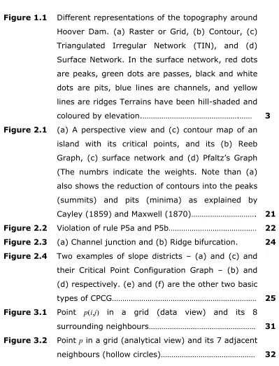
Figure 1.1 Different representations of the topography around Hoover Dam. (a) Raster or Grid, (b) Contour, (c) Triangulated Irregular Network (TIN), and (d) Surface Network. In the surface network, red dots are peaks, green dots are passes, black and white dots are pits, blue lines are channels, and yellow lines are ridges Terrains have been hill-shaded and

coloured by elevation.……….…… 3

Figure 2.1 (a) A perspective view and (c) contour map of an island with its critical points, and its (b) Reeb Graph, (c) surface network and (d) Pfaltz’s Graph (The numbrs indicate the weights. Note than (a) also shows the reduction of contours into the peaks (summits) and pits (minima) as explained by Cayley (1859) and Maxwell (1870)………. 21 Figure 2.2 Violation of rule P5a and P5b……… 22 Figure 2.3 (a) Channel junction and (b) Ridge bifurcation. 24 Figure 2.4 Two examples of slope districts – (a) and (c) and

their Critical Point Configuration Graph – (b) and (d) respectively. (e) and (f) are the other two basic

types of CPCG……… 25

Figure 3.1 Point p(i,j) in a grid (data view) and its 8

surrounding neighbours……… 31

Figure 3.3 Decomposition of a degenerate pass (Modified from Takahashi et. al, 1995). Figure shows the neighbours and their heights. Higher neighbours are placed inside a grey region. (a) The original neighbour list, (b) the reduced neighbour list, (c) the list in the first turn of the loop in the algorithm, and (d) the final set of neighbours which will define

the pass………. 33

Figure 3.4 Critical points of the surface and the configuration of their eigenvalues and eigenvectors. R1 and R2 are the real parts of the eigenvalues………. 37 Figure 3.5 (a) Elliptic, (b) hyperbolic and (c) parabolic conic

sections with their semi-axes idetified (After Wood, 1998). A planar case is not considered here………….. 39 Figure 3.6 Three possible intersection cases between

(circular) region of interest and conic section’s semi-axes (After Wood, 1998). (a) Two axes intersect with region – pits, peak or pass, (b) one axis intersects with region – channel or ridge and (c) no intersection – planar……….………. 39 Figure 4.1 Generalisation Lineages and Stages in spatial data

structures………. 42

Figure 4.2 A hypothetical island and the (yo – zo)-contraction and (yo – zo)-contraction of its surface network. The numbers in the square brackets in (a) denote the height of the critical points and x is the

surrounding pit………. 46

Figure 4.3 (a) Hypothetical topographic surface and its (b) surface network. Blue contour represents the

surrounding pit………. 53

Figure 4.4 (a) Topography around the Latschur Mountains in the Carinthia Region, Austria and (b) its surface

Figure 4.5 Graphical User Interface of the Surface Topology Toolkit application with the controls for the

contractions.….………. 54

Figure 4.6 Comparison of the effectiveness for selection of points in the surface network (a) between maximum of elevation difference criterion (b) and maximum of edge length criterion (c). Note that criterion (b) selects a long ridge due to its low drop

in elevation (350)………. 57

Figure 4.7 Comparison of the effectiveness for selection of points in a (a) surface network, between (b) sum of elevation difference criterion and (c) valency criterion, showing how criterion (b) can mislead about the ridge/channel crossings. Numbers at peaks in (a) are sum of elevation differences and their valency (in parentheses)………..………. 57 Figure 4.8 Generation of an artificial valley inside the dotted

region of the Latschur surface network……… 58 Figure 5.1 Comparison of the dumbness and uncertainty in

spatial data structures……… 61

Figure 5.2 Comparison between the current and surface network enhanced visualisation of the dynamism in the geopotential height over Europe………. 63 Figure 5.3 Intervisibility calculations in a part of Isle of Man,

List of Tables

Table 1.1 Sequence of the “interdisciplinary” research on

surface networks……… 8

Table 3.1 Criteria for classification of critical points in the

eight-neighbourhood method……….. 31

Table 3.2 Criteria for classification of non-degenerate critical

points based on delaunay triangulation……….. 32 Table 3.3 Morphometric Features descibed by second

Chapter 1

Introduction

1.1 Surface Information Encapsulation

The desire to understand and exploit the structure of continuous surfaces is a common aim to researchers in a range of disciplines. A few examples of the varied surfaces forming an integral part of modern subjects include terrain, population density, surface atmospheric pressure, physico-chemical surfaces, computer graphics, and metrological surfaces. However, with an increasingly multispectral and highly dense data (surfaces in this case), researchers want to be able to filter out redundant observations. These aims (more information but less data volume) seem to contradict each other. However, a right balance between the volume of the data and the information content in the data is an essential requirement to make our analyses (human or robotic) fast and to keep our data storage usage to a minimum. In addition to the understanding, considerable efforts are also spent to produce computing methods to perform data processing automatically.

contains more information. What is important to note here is that there is an inevitable demand for data structure designs and computing algorithms to achieve a satisfactory DI/DV.

(a) (b)

(c) (d)

As mentioned earlier, these varieties of the critical point-critical line data structures could have different construction but their “Surface Topology” has the same set of components. Thus, based on this similarity between these data structures and for the sake of simplicity, we propose here author the following terms are used,

- “Surface Network” for the spatial representation, and - “Surface Network Graph” for the graph representation,

for all data structures constructed with critical points and critical lines. Note that this definition excludes Triangulated Irregular Networks (TIN) because they contain both the critical and ordinary set of points in their structure. The above-mentioned convention will be used in the following parts of this report. However, the author realises that this proposal can only be sensible if there were to be a universal standard on the structure and implementation of surface networks. A specific aim of this research is to combine the aims and methods of various disciplines on this subject.

1.2 Fundamental issues in Surface Topology

There are many other types of surface topological data structures in GI science and other subjects. Wolf (1993) has given a review of some prominent surface topological data structures. In order to achieve a thorough grounding for this work, it is essential to define rigorously those aspects of surface topology and topological data structures which are used to describe surfaces.

Q1. Why should we have surface topology based data structures?

• Topological connections are a much more efficient way to access a spatial database. In this case, surface networks provide a more natural and thus intuitive control on the structure of the surfaces.

• Components in a topological data structure are interdependent and linked. Thus, these data structures can be used for applications that require uniform and controlled response from the entire surface such as morphing in computer graphics and erosion modelling. For example, in the case of surface (represented as contours) generalisation, a common problem in approaches based on line-simplification is the intersection of contours after simplification. However, in the case of a surface network representation of the surface, the use of formal topological simplification prevents the generation of an unrealistic surface after generalisation (Wolf, 1984).

• Surface topology is found more useful for the visualisation of surfaces especially 3D surfaces. It is because as it does not involve the complications of deciding the appropriate colour mapping or contour interval or the density of triangles (in case of TIN) (Helman and Hesselink, 1991; Bajaj and Schikore, 1996).

• As the surface networks are translation- and rotation- invariant they also forms an ideal mechanism for correlating and co-registering surfaces (Bajaj and Schikore, 1996).

Q2. What should the data structures for the surface topology attempt to describe?

• A common expectation from the topological data structures is that they should provide a unified global description of surface. A global description would ensure a sympathetic response in the whole surface if a change occurs in one part of the data structure. Thus, giving a formal control on the continuity of materials and processes that exists in nature as well.

• The data structure should be able to represent most surfaces i.e., both fluvial and non-fluvial (with no or incomplete set of pits, peaks, and passes).

•

Q3. Which surface features should be considered as most important to be included in the surface topology data structures?

Various surface specific features have been proposed to represent the surface. The choice was largely based on the specific applications for which the surface was being modelled. The choice of surface specific features for the framework of surface topology is very essential, as it will decide the following important factors:

• Resemblance to a real surface: The combination of surface specific features selected for surface topology should be able to describe most of the surface forms. However, the more detailed set of surface specific features are selected, the more difficult it will be to handle the data structures.

1.3 Outline of the Report

Surface Networks have received intensive research inputs from researchers especially in computer science (vision, graphics), geographic information science (terrain modellers) and, to a limited extent, by social scientists. The research on surface networks can be broadly divided into four main areas namely the Design (i.e., data structure model), Extraction (Automated, Digital), Generalisation, and Applications. The chronological sequence of research in these areas is shown in Table 1.1. The report is also divided into four parts based on the research areas, namely Theoretical or Design of Surface Networks (Chapter 2), Extraction (Chapter 3), Generalisation (Chapter 4), and the Applications (Chapter 5). These chapters are mostly self-contained description on these areas and include a conclusion either during the description or at the end of the chapters. This has been done to ensure a consistency of thoughts.

Chapter 2 presents a review of the various surface network data structures with insights into their design and applications. This chapter will propose properties expected in a general design of surface network in order to be applicable for most kinds of two-dimensional surfaces.

Chapter 3 focuses on the automated extraction of surface networks. This will involve the treatment of issues such as scale, feature identification and generation of a consistent topology. Three techniques of the extraction namely manual, triangulation and surface fitting will be described in details.

Surface Network Research Areas

Researcher(s) Design Extraction Generalisation Visualisation

Reech (1858)* x -- -- --

Cayley (1859)^ x -- -- --

Maxwell (1870)^ x -- -- --

Morse (1925)* x -- -- --

Reeb (1946)* x -- -- --

Warntz (1966)^ x -- -- --

Morse (1966)^ x -- -- --

Pflatz (1976)*^ x x x x

Mark (1977)^ x ? x --

Nackman (1984)* x x -- --

Wolf (1984)^ x -- x x

Takahashi et. al (1995)*^ x x -- x

Rana (2000)^ -- -- x x

Biasotti et. al (2000)*^ x x -- x

Wood, Rana (2000)^ x x x x

Table 1.1 Sequence of the “interdisciplinary” research on surface networks. ^ indicates a research based on terrains as the example of surface and * indicates a research based on a mainly mathematical treatment of surfaces.

comments on the regeneration of the surface around the topological adjustments.

1.4 Domain of the Report

Until now in the report, the term surface was used loosely to indicate continuous surfaces in n-dimensions. However, in this research a surface has the following strict definition:

- Surface is a twice continuously differentiable function, whose each point (x,y) is associated with its scalar property i.e., z = f (x,y) and

Chapter 2

The Design of Surface Networks

2.1 Origins

From early in various academic fields, attempts have been made to parameterise surfaces into frameworks woven around the geometrical and topological relationships of the fundamental features of the surface. Efforts have taken place in disciplines such as physical and social geography, computer science (particularly graphics and vision), medical sciences, metrology, physics and others, in which the data and output is often a continuous surface. The aim of this chapter is to discuss the various surface network data structures especially around their capabilities to represent the surfaces accurately. In the following text a brief description on the sequence of events related to the developments of surface networks will be given. The details on the individual events are provided thereafter.

The most crucial thought, which was instrumental in the surface network field, was the recognition of the fundamental features. Fundamental features are characteristic features, which are common to all surfaces and contain sufficient information to construct the whole surface, thus taking away the need to store each point on the surface.

Mark (1977) reported that Reech (1858) was perhaps the first to discuss the critical points on a closed surface. It was soon followed by Cayley (1859), who proposed the subdivision of topographic surface into a framework of summits, immits, knots, ridge lines and course lines.

passes, number of immits (also called bottoms) and number of bars. He also described the partition the topographic surface into “Hills and Dales” based on these features.

In contrast, Morse (1925) proved the same relations between the number of peaks (summits), number of passes (bars), and number of pits (immits) based on differential topology. In general, Morse proposed formal relations between the critical points in an n-dimensional surface, which is known as the Critical Point Theory or Morse Theory. The generic nature and wide applicability of Morse Theory led to the expansion in the interest in the critical points of surfaces amongst various disciplines.

In a significant related development, Reeb (1946) proposed representing the splitting and merging of equi-height contours (i.e., a cross-section) of a surface as a graph. Now as the contours close at the pits and the peaks, and split at the passes, therefore the vertices of this graph, now called Reeb Graph, are the critical points of the surface. The edges of the Reeb Graph turn out to be the ridges and channels. The Reeb Graph was particularly useful because unlike the description of the relationships critical points on the surface given in the Morse Theory, it addressed the embedding of the critical points on the surface.

Warntz (1966) revived the interest of geographers and social science researchers into critical points and lines when he applied the “Hills and Dales” idea for socio-economic surfaces, referred to as the Warntz Network (Mark, 1977).

Tree in details, does not mention Reeb Graphs. As in the case of Reeb Graph, the vertices of such a contour tree are the peaks, pits and passes.

After about a decade Pfaltz (1976) combined Morse Theory inequalities and Warntz Network in a formal graph-theoretic data structure called Surface Network (also called Pfaltz’s Graph - coined by Mark, 1977). Since he was in the computer science field, his work attracted the attention of researchers in three-dimensional surfaces such as in medical imaging, crystallography (Johnson et. al, 1999; Shinagawa et. al., 1991) and computer vision (Koenderink and Doorn, 1979). Pfaltz also proposed a graph-theoretic method called homomorphic contraction for generalising the Pfaltz’s graph and made the first attempt at the automated generation of surface networks.

Mark (1977) proposed a pruning of the contour tree to remove the nodes (representing contour loops) which do not form the critical points, i.e., the vertices, of the contour tree, and called the resultant structure “Surface Tree”. This essentially reduces the contour tree to the purely topological state of a Pfaltz’s graph. It is easy to realise that the Reeb Graph, Pfaltz’s Graph and Surface Tree have fundamental similarities and are actually inter-convertible (Takahashi et. al, 1995).

Nackman (1984) proposed a new construction for the graphs of critical points, called the “Critical Point Configuration Graph (CPCG)”, to be a surface network under more general conditions than those in the Pfaltz’s graph. In most simple terms, the CPCG is made up of four basic combinations of the critical points called the Slope Districts (areas of overlap between Hills and Dales).

The next major work in the Pfaltz’s Graph lineage was by Wolf (1984), who introduced more topological constraints for the Pfaltz’s graph to be a consistent representation of the terrain. He proposed assigning weights to the critical points and lines to indicate their importance in the surface and thus he proposed the name “Weighted Surface Network” for the Pfatlz’s graph. He demonstrated new weights-based criteria and methods for the contraction of the surface networks. He, however, performed a manual extraction of surface network from contour maps.

Interlocking Ridge and Channel Network (Werner, 1988), Hills and Dales, Contour Tree, Surface Tree, and Pfaltz’s Graph. Sadly, although interesting, the idea did not advance beyond the Entity-Relationship Model of the data structure.

A major contribution in surface networks came from Takahashi et. al (1995), who combined the Morse Theory and the Reeb Graph ideas and proposed robust algorithms for the automated extraction of a consistent Surface Network from DEM. A unique aspect of his work was that he used a triangulation based feature detection method to extract the critical points.

On the contrary, Wood (1998), Wood and Rana (2000) attempted to extract the critical points using a polynomial based feature extraction technique with limited success. The advantage of a polynomial-based detection is that it could be adjusted to extract features at various scales unlike the triangulation-based technique, which is restricted to a fixed scale. Rana (2000) discussed the characteristics of Wolf (1984)’s generalisation criteria and proposed an arbitrary user-defined contraction for surface networks.

Now the stage has been set up to describe each of the above-mentioned work in details. The work of Reech (1858) was not available to the author at the time of writing this report so it will not be discussed.

2.2 Surface Network Data Structures

2.2.1 Contour and Slope Lines

Cayley (1859) described the configuration of terrains based on the arrangement of contour lines and slope lines.

reduce to a point, which is called Immit. At some points in the terrain, a contour line may meet three contour lines of the equal elevation. At these points, the surface is horizontal, and one descends in the backward and forward directions while the other ascends in right and left directions. These points are called Knots.

The indicatrix at a summit and immit is an ellipse except in the case when the summit or immit is an umbilicus – the indicatrix then is a circle. Hence in the case of an elliptic indicatrix, all slope lines except one intersect direction of least curvature of the ellipse. The remaining contour lines intersect the contour lines of maximum curvature of the ellipse. The indicatrix at a knot is a hyperbola and therefore the contour lines in the neighbourhood of a knot are similar and similarly situated concentric hyperbolas. At the knot, there are two orthogonal slope lines, which bisect two opposite contour line hyperbolas. This pair of slope lines is the Ridge and Course lines. A knot is a point of minimum elevation for a ridge line while it is a point of maximum elevation for a course line. A ridge line would reach from a knot to summit and a course line would reach from an immit to another immit via a single intervening knot. However, the course line can also arrive at the sea-level contour without reaching another immit. The ridge line or course line may start and end at the same summit or immit respectively, thus forming a closed curve.

2.2.2 Hills and Dales

Maxwell (1870) developed the Cayley (1859) description of the Surface Topology of terrains. Like Cayley (1859) he proposed his ideas based on an elevated surface surrounded by a depression.

meeting, which is called a Pass, cuts off two regions of elevation from one region of depression. Thirdly, the regions of elevation and depression are finally reduced to points, which are called Summits or Tops and Immits or Bottoms respectively.

Given the above ways of generation of the features, Maxwell (1870) derived relations between the number of summits, passes, immits and bars. Every new region of elevation produces a pass. A summit is produced when every new region of elevation is reduced to a point. Therefore, since the whole surface of the earth is a region of depression, the number of summits, S, is one more than the number of passes, P, i.e.,

S = P + 1 ….(2.1)

Similarly, with every new region of depression, a bar is produced and an immit develops when the region of depression is reduced to a point. Therefore the number of immits, I, is one more than the number of bars, B., i.e.,

I = B + 1 ….(2.2)

A pass or a bar can be called a single, double, or n-ple according to two, three, or n+1 regions of elevations or depressions meeting at a point.

He added that these rules apply to any function of two variables. The summits are the maxima and the immits are the minima. Therefore, based on the two eqs. 2.1 and 2.2, for this function with number of maxima, p, and number of minima, q, there are

p + q – 2 ….(2.3)

cases of stationary values, which are neither maxima nor minima. He extended this relation, in an interesting way, to function of three variables, which is beyond the scope of this report.

Geomorphologically and analytically (as expressed by eq. 2.3), the bars and passes are the same features, called saddles or passes. The points of stationary values which are neither maxima nor minima are in fact the saddles, which gives us the following important relation between the number of summits, S, number of immits, I, and number of passes, P,

I – P + S = 2 ….(2.4)

Slope lines are lines that are everywhere at right angles to the contour lines. All slope lines, except two, when ascending generally reach a summit and when descending end at an immit. The exceptional two slope lines reach a pass or a bar. The surface is divided into two types of Districts (areas of surface). These are the Dales or Basins, whose slope lines converge at the same immit and the Hills, whose slope lines originate at the same summit, which are called Hills. Dales and Hills are partitioned by Watersheds and Watercourses respectively. A watershed can be drawn from a pass or a bar by tracing the slope line from the maxima connected to this pass (bar) until it reaches a summit. A watercourse is similarly a slope line starting from the minima connected to a pass (bar) and ending at an immit. Lines of watershed never reach an immit and lines of watercourse never reach a summit.

Based on the deductions above the total number of summits, S, on the whole surface is

S = 1 + p1 + 2p2 +…+ (n-1)pn-1 ….(2.5)

where p1 is the number of single passes, p2is the number of double passes and so on, and n is the maximum number of regions of elevation meeting up at the summits. The total number of immits, I, is

I = 1 + b1 + 2b2 +…+ (n-1)bn-1 ….(2.6)

where b1 is the number of single passes, b2is the number of double passes and so on, and n is the maximum number of regions of depression meeting up at the immits. Therefore the number of watersheds, W, will be

W = 2 (b1 + p1) + 3 (b2 + p2) + ...+ (n+1) (bn-1 + pn-1) ….(2.7)

where n is the order of pass and bar i.e., single, double and so on. The number of watercourses is similarly defined.

Now according to the Listing’s rule for finding the number of faces, P – L + F – R = 0 ….(2.8)

where P is the number of points, L is the number of lines, F is the number of faces and R is the total number of regions. Here R = 2, viz. the earth and the surrounding spaces, hence

F = L – P + 2 ….(2.9)

represents watercourses, then P will equal to the total number of immits, passes and bars and F will be the number of Hills or i.e., the summits. Finally, if we assume that L is equal to the total number of lines, and P is equal to the total number of points then F, the total number of natural districts i.e., the hills and dales together, is equal to the total number of watersheds and watercourses or the total number of summits, immits, passes and bars minus 2.

Warntz (1966) reiterated these ideas and proposed their use in understanding socio-economic surfaces and spatial flows. For an example he used population potential surface of USA and demonstrated various applications of Hills and Dales in transport network density, movement of money etc.

2.2.3 Critical Point Theory

The first purely mathematical treatment of surface networks came from Morse (1925). He considered the “critical points” of a sufficiently smooth function f defined over an arbitrary n-dimensional manifold M where f satisfies appropriate conditions on the boundary of the manifold.

Milnor (1963) is a widely referred book for a background reading on Morse Theory but this book is out of print and is not available easily ( and was not available to the author either). Three good alternative sources are Pfaltz (1978), Takahashi (1996) and the Encyclopaedia Britannica.

The conditions and definitions on the surface function f are:

- f is sufficiently smooth if f ∈ C2 _{i.e., it has continuous 2}nd _derivatives. Thus, it is possible to calculate the curvature at each point on the function so cases like overhangs and lakes do not exist,

- A point p ∈ M is a critical point of f if δf(p) = 0 i.e., the 1st _partial derivative of f vanishes at p or f is “locally flat” at p.

- For all points b on the boundary f(b) > f(i) where i is an interior point. - All critical points of f are non-degenerate i.e., the matrix H(f) of the 2nd

H(x, y) =

y

x f

f f

δ δ

δ _….(2.10)

- The index of the critical point p of f is the number of negative eigenvalues of the Hessian matrix at p.

In this work, the dimension of the manifold is 2, therefore the indices of the critical points are from 0 to 2. It turns out that the peak of the function f has the index 2, a pass has the index 1 and a pit has the index 0.

- The function f on M is called a Morse function if it has no degenerate critical point. An example of a degenerate critical point in terrain is the monkey saddle. A point at a monkey saddle although locally flat has a non-singular Hessian matrix.

With these conditions and premises for the function f and its critical points, Morse related the number of critical points of f with the topology of the Manifold. The details of the comparison are not specifically relevant to be provided here. But the following inequalities derived by him for a 2-dimensional sphere (f is assumed to be a part of the sphere) are important to be noted here:

P0

≥

1

≥

1

where P0, P1 and P2 denote the critical points of index 0,1 and 2 respectively. As mentioned, earlier in the discussion, in the case of 2-dimensional function they correspond to pits, passes and peaks respectively. Note the similarity between the sophisticated eq. 2.13 and the simpler eqs. 2.4 and 2.9. These inequalities are a simple example of Critical Point Theory or Morse Theory by Morse (1925).

In later works, Morse demonstrated the use of these relations in the understanding of various surfaces such as in physics, biology, and economics and thus encouraged the wide spread use of the Morse Theory

Secondly, it is well known that surfaces, especially terrains do contain abundant degenerate points. Therefore, terrains are not ideally a Morse function by definition. However, the potential advantages of storing the “structure of a surface” in a critical point framework are very attractive and it will be shown in the next chapter that degenerate points can be hypothetically “decomposed” into a non-degenerate point.

2.2.4 Reeb Graph and Contour Trees

A Reeb Graph (Reeb, 1946) is a graph which represents the splitting and merging of equi-height contours (Takahashi et. al, 1995). The original article by Reeb (1946) is in French but formal discussions of his ideas in English are given by Takahashi et. al (1995), Takahashi (1996) and Biasotti et. al (2000).

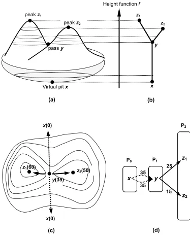
The following description of the Reeb Graph is largely taken from Takahashi et. al (1995). For a function f representing the height of a terrain, its Reeb Graph is obtained by identifying points p and q if the two points are contained in the same connected component on the cross-section of the surface at the height f (p) = f (q). Thus, a cross-sectional contour is represented as a point of the edge of the Reeb Graph (Fig. 2.1). As explained in section 2.2.1 contours converge or diverge at the critical points, therefore the vertices of Reeb Graphs represent the critical points of f. Fig. 2.1a shows an example of a mountain and its critical points and Fig. 2.1b is its corresponding Reeb Graph. The combination of the Reeb Graph with the Morse Theory could be one formal way of representing the topological configuration of the critical points on the surface as a single data structure. Biasotti et. al (2000) has developed the Reeb Graph to model terrains, and it is referred as the Extended Reeb Graph (ERG). One of the main characteristic of ERG is that it uses the areas around critical points, called critical areas, as that allows a better reconstruction of the surface. Biasotti’s work is an example of widely discussed issue in geomorphometry of whether a peak is actually a point or an area.

2.2.5 Surface Network or Pfaltz’s Graph

Pfaltz (1976) was the first researcher who proposed a formal topological data structure for surfaces based on the combination of the Critical Point Theory and the theory of Hills and Dales. He essentially added the missing connectivity between the critical points of a surface (which is a Morse function) in the Critical Point Theory by using the relationships defined between the critical points in the theory of Hills and Dales. He proposed that the relationships between the critical points can be represented by a tripartite (three sets of critical points) directed graph, which he called the Surface Network, also known as Pfaltz’s Graph (Mark, 1977). For example for the surface in Fig. 2.1a, its surface network and Pfaltz’s Graph are shown in Fig. 2.1c and Fig. 2.1d respectively. However, not all such tripartite graphs can represent a real surface (Pfaltz, 1976; Wolf, 1984). A weighted, directed, tripartite graph W = (P0, P1, P2; E), where P0, P1, P2 are

the three vertex sets representing the sets of all pits, passes and peaks, respectively, while E is the set of all edges, is termed a (weighted) surface network (WSN) if

P0: W is planar.

This means that an intersection of edges for instance an intersection of ridges and channels is not allowed. This is natural because except at the critical points, there can only be one type of slope line passing through one point.

P1: The subgraphs [P0, P1] and [P1, P2] are connected.

This means that channels connect pits and passes, and ridges connect peaks and passes.

P2: |P0| - |P1| + |P2| = 2

Height function f

peak z1

peak z2

pass y y

z2

z1

Virtual pit x x

(a) (b)

x(0) P2

y(35)

z2(50)

z1(60)

z

z

x y

35 P1

15 25 P0

x(0)

(d) (c)

P3: For all y ∈ P1, id(y) = od(y) = 2 where y = pass, id(y) = in-degree of y, od(y) =

out-degree of y.

This means that exactly two channels and exactly two ridges emanate thus excluding the existence of degenerate passes. As can be seen in nature, this property is most often violated for example in the case of channel junctions and ridge bifurcations. Pfaltz (1976) suggested that these points could be “decomposed” into normal critical points. Wolf (1990) and Takahashi et. al (1995) proposed solutions, which will be discussed later in this section and in the next Chapter.

P4: val(x, yi) = val(yi, z) = 1 implies that there exists yj ≠yi such that (x,yj),

(yj,z) ∈E, where x = pit, y = pass, z = peak and val = valency.

It guarantees that if there is a path from pit x via pass yi to peak z, which

consists only of edges with valency one, then there exists another path from pit x to peak z via a distinct saddle yj.

P5a: (x,y) is an edge of a circuit in the bipartite graph [P0,P1] iff val(y,z) ≠ 2 for

all z∈ P2

P5b: (y,z) is an edge of a circuit in the bipartite graph [P1,P2] iff val(x,y) ≠ 2 for

all x∈ P0

This property asserts that a configuration as shown in Fig. 2.2 is impossible.

y

z _x

Figure 2.2 Violation of rule P5a and P5b.

P6: w(ei) > 0 for all ei ∈E

This means that all the edge weights must be greater than zero. For instance, if h(x0), h(y0) and h(z0) represents the elevations of a pit, pass and

peak, respectively, then the weight of a channel is h(y0) - h(x0) and the

P7: For all x∈ P0 , yi, yj∈P1 , z∈P2 and (x,yi), (x,yj), (yi,z),(yj, z) ∈ E holds

w(x,yi)+w(yi,z) = w(x,yj)+w(yj,z)

This means that for all paths from pit x to peak z the difference in elevation is the same, no matter which saddle point is passed.

P8a: If val(x,y) = 2 with ei1=(x,y) and ei2 =(x,y) then w(ei1) = w(ei2)

P8b: If val(y,z) = 2 with ei1 =(y,z) and ei2 =(y,z) then w(ei1) = w(ei2)

This means that all channels from a pit to a pass have the same difference in altitude; the same holds for ridges, too.

Wolf (1984) developed Pfaltz’s Graph and proposed weights to be assigned to the critical points and lines to indicate their importance in the local or global structure of the surface. He thus called the new form a Weighted Surface Network (WSN). Although surface networks are an abstraction of surfaces, they could still have redundant information. Pfaltz (1976) proposed a graph-theoretic method of simplification of surface networks called Homomorphic Contraction, which can remove redundant vertices and edges but still preserve the above-mentioned topological properties of the surface network. Wolf (1984) developed Pfaltz’s ideas on homomorphic contraction and introduced the use of weights and various criteria for the contraction. More information on the contraction is explained in Chapter 4, which describes the generalisation of surface networks.

It is evident from Fig. 2.1c,d that the surface networks are purely a topological data structure. However, as Wolf (1993) commented an ideal data structure for a surface should be able to describe both the topological and geometrical properties of the surface. This issue has been addressed in mainly two ways.

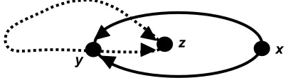
be represented as an infinitesimally close pair of pit-pass and pass-peak, respectively (Fig. 2.3). In the case of junctions and bifurcations, an arbitrary low weight can be assigned to indicate their proximity, for example Wolf (1990) used a value of 2.

Bifurcation Junction

(b) (a)

Peak

Pass

Pit

Channel

Ridge

Figure 2.3 (a) Channel junction and (b) Ridge bifurcation.

Takahashi et. al (1995) proposed the use of Reeb Graphs to reconstruct the topography as they store information about the hierarchy of the contours. He found that it was easy to construct the Reeb Graph from the surface network, as it will be very time consuming to detect the topological changes in the cross-sectional contours.

The next chapter will present the slope lines (ridges and channels) based approach (Wood and Rana, 2000) to maintain the topographic appearance and the topological virtues of the surface networks.

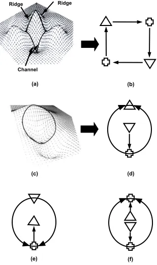
2.2.6 Critical Point Configuration Graph

Ridge Ridge

Channel

(a)

(b)

(c) (d)

(e) (f)

using differential equations and Morse Theory that the surface i.e., the CPCG, under reasonable assumption, contains four basic cycle types or slope districts (Fig. 2.4b,d,e,f). Nackman, however, did not propose how these slope districts could be conglomerated or paste together to form a single representation of the surface. This was perhaps one of the main reason for the lack of wide interest in CPCG (Recently revived by Rosin, 1995; Scott, 1998). In addition, as can be seen in the slope district at lower right (Fig. 2.4f), a pass can connect to pass with no intervening peaks or pits, which violates the rules laid by the theory of Hills and Dales for the ridge lines and course lines. Pfaltz (1978) reported that it is easy to create such surfaces mathematically (Morse, 1964) but remained uncertain if they could be used for terrains.

2.3 Summary

In conclusion for this chapter, it has been found that a generic treatment is still required to promote the surface network for wide and indiscriminate use. The following issues need to be addressed:

- Due to their design requirements, current implementations of Surface Networks have been restricted to surfaces with fluvial features (i.e., must have ridges, channels, peaks, passes, and pits). However, a number of surfaces have biased topography such as in glaciated or karstic terrains or features may be absent e.g., flat surfaces. Takahashi (1996) believes that the biased surfaces are cases of degenerate critical points and the presence of degenerate points leads to the violation of Euler criterion or Mountaineer’s equation. His approach for handling degenerate points has been discussed in the next chapter.

although unlike surface network it would not provide any insights into the structure of the surface. However, it is also important to note that the approximation uncertainty will also usually be higher with the use of surface networks for discrete data.

Chapter 3

Extraction of Surface Networks

3.1 Introduction

The process of accurate and indiscriminate extraction of a surface network from its surface lies in the middle of the surface network model and its use in practise. Therefore, the extraction will set the potential usability of the surface network data structures. In fact, the original motivation of this PhD was the opportunity of new ideas in the automated extraction of surface networks. It is well known that the theoretical ideas are often not easy to be implemented in practical computing. There is generally some level of compromise between the accuracy and the processing efficiency. For example, in the case of surfaces, a discrete DEM is a preferable representation against a realistic polynomial representation because it is easier to manage and generate it, although the uncertainties with the discrete representation could be significant.

3.2 Surface Network Extraction Methods

Most simply, the generation of a surface network involves two steps – (i) extraction of the critical points and (ii) connecting them with the critical lines. However, the methods used for these two steps are still far more satisfactory. Two main concerns in the automated generation of surface networks are scale dependency and subjective feature definitions.

The issue of scale dependency is a multi-faceted and intensively studied topic across the academics. Various definitions and classifications have been proposed for scale and a number of books are dedicated in computer science (Lindeberg, 1994), earth sciences (Quattrochi and Goodchild, 1996) and social sciences on the determination and effects of scale in the processing. The basic issue, which concerns us, is that the features, objects and information exist across a range of scales, whose arrangement may and may not be hierarchical. At any one instance, our computing routines can detect features that fit into the fixed search window (kernel etc.). Therefore, the feature extraction could only be valid for the current scale but not as a true (natural) representation of the surface. In order to detect the scale, there have been attempts to model surface as fractals (Fels and Matson, 1996; Emerson and Quattrochi, 2000), wavelets (Starck et. al, 1998) or a simple hierarchical subdivision of surface (Csillag, 1996).

1994). However, most surfaces and images have a mix of features of different topological dimensions. In other words, the structure of the surface or image is actually made up of features of different topological types. For instance, in the case of surface networks, both the critical point and lines are important but they belong to different topological classes. The current algorithms do not take into account that different topological objects are expressed differently under different scales. For instance, points tend to be lost more quickly compared to lines over decreasing scales (zooming out). The conceptual issues such as “What is scale” and “What is the right scale of the surface?” also need to be addressed (Montello and Golledge, 1998).

Numerous methods and models have been proposed to characterise the critical points and lines. There is no consensus on the feature extraction technique but methods and algorithms are becoming more sophisticated (complicated) and universally available. The success of the algorithms depends on the critical point model i.e., eight neighbour methods or surface fitting and its scale dependency. For instance, some methods extract features in certain surfaces better than in other surfaces and some methods extract features better over only certain scales.

The main stress of this work so far has been to understand the various techniques and to put more efforts on the perceptual organisation of the features, building a topologically consistent surface network in this case. The following part of this chapter will describe some prominent methods for the automated, except one, extraction of surface networks.

3.2.1 Manual Extraction

may have followed an optimised methodology to extract a consistent surface network.

3.2.2 Triangulation

3.2.2.1 Definitions and Methodology

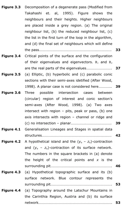
Takahashi et. al (1995) proposed a modified version of the eight-neighbour method based detection of the critical points (Peucker and Douglas, 1975) for grid surfaces. The eight-neighbour method compares the height of a point, p(i,j), with its eight neighbours in a 3 x 3 square surrounding p (Fig. 3.1) and classifies the point as a critical point based on the criteria in Table 3.1.

i +1 , j i +1 , j -1

i , j -1

i –1 , j -1 i –1 , j i –1 , j +1

i , j +1

i +1 , j +1

p (i,j)

Figure 3.1 Point p(i.j) in a grid (data view) and its 8 surrounding neighbours.

peak |∆+| > Tpeak |∆-| = 0 Nc = 0 pit |∆-| > Tpit |∆+| = 0 Nc = 0 pass |∆+| + |∆-| > Tpass Nc = 4

|∆+|

|∆-|

Nc Teak Tpit Tpass

The sum of all positive height differences between the point and its 8 neighbours

The sum of all negative height differences between the point and its 8 neighbours

The number of sign changes associated with the point Threshold height for a point to be a peak.

Threshold height for a point to be a pit Threshold height for a point to be a pass.

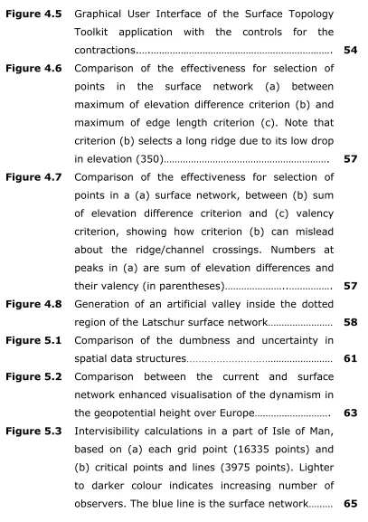
eight-Takahashi et al. (1995) showed that the eight-neighbour method based detection is subjective to the value of the threshold and this ambiguity could cause the loss of the Euler Formula property also called the Mountaineer’s Equation i.e., pits – passes + peaks ≠ 2. He suggested that in order to satisfy the Euler formula the contour changes should be determined according to the neighbour heights and not according to the threshold. He suggested the use of the Delaunay triangulation (Guibas and Stolfi, 1985) to triangulate the 3 x 3 square, centered at p, and

p

Figure 3.2 Point p in a grid (analytical view) and its 7 adjacent neighbours (hollow circles).

determine only the adjacent points (amongst the 8 surrounding neighbours) of p (Fig. 3.2). The point is then classified according to the criteria given in Table 3.2.

peak |∆+| > 0 |∆-| = 0 Nc = 0

pit |∆-| > 0 |∆+| = 0 Nc = 0

pass |∆+| + |∆-| > 0 Nc = 4

Table 3.2 Criteria for the classification of non-degenerate critical points based on Delaunay triangulation.

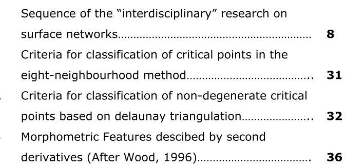
100 p 100 p 100 p 100 p (d) 110 104 93 86 p6 p5 p3 p2 (c) 110 104 93 89 106 86 p7 p6 p5 p3 p1 p2 (b) 110 104 93 89 106 86 p7 p6 p5 p3 p1 (a) 110 103 104 93 89 106 86 p7 p6 p5 p4 p3 p1

p2 p2

Figure 3.3 Decomposition of a degenerate pass (Modified from Takahashi et. al, 1995). Figure shows the neighbours and their heights. Higher neighbours are placed inside a grey region. (a) The original neighbour list, (b) the reduced neighbour list, (c) the list in the first turn of the loop in the algorithm, and (d) the final set of neighbours which will define the pass.

The algorithm to decompose a degenerate pass by Takahashi (1995) is unique and noteworthy. The steps are as follows :

(i) Generate a counter-clockwise (CCW) list of the adjacent neighbours of this pass, which in this case is {p1, p2, p3, p4, p5, p6, p7} (Fig. 3.3a). (ii) Divide this list into an upper sequence, which has the higher

is higher in the sequence { p3, p4}. Note that if the list has more than one neighbour then the reduced list begins with a lower neighbour to ensure that the four alternating upper and lower neighbours at the pass are selected correctly. Also it can be seen from the reduced list that ther are 6 sign changes thereforre, the number of denegerate passes m is 2.

(iii) Put all the elements of the reduced list except the first two i.e., {p5, p6, p7, p1}, in a trailing list to further reduce the neighbours list.

(iv) Select the last four elements i.e., {p5, p6, p7, p1}, of the trailing list as representative neighbours. Remove the last two elements, which are {p7, p1} in this case, of the representative neighbours, from the trailing list.

(v) Repeat steps (iii) – (iv) untill the trailing list is reduced to a lower and a upper neighbour of the pass, which in this case are {p7, p1} and were easily achieved. The final neighbours list of the decomposed pass has the first two elements of the trailing list and the two elements remained after step (v) thus in this case the final neigbhours of p are {p2, p3, p5, p6}.

The methodology to connect the points is quite simple. It is based on the assumption that a ridge line is the line of steepest ascent from a pass while a channel is the line of steepest descent. Therefore, the ridge (channel) line is traced by moving to the highest (lowest) neighbour and repeating the tracing until a peak (pit) or the boundary is reached.

Takahashi et. al (1995) proposed that the above methodology would successfully extract a consistent surface network. However, we have some doubts, which will be shown in the next section.

3.2.2.2 Discussion

current method of triangulation can be extended to detect larger features.

(b) Limitations of feature classification:

- In order to avoid the inaccuracies related to the mathematical division of numbers, Takahashi et al. (1995) preferred the use of linear interpolation (Delaunay triangulation) to smooth surface (quadratic, cubic) fitting based methods to classify the points. See Wood (1996, 1998) for the disadvantages of the linear interpolation of heights for the classification of critical points and the extraction of surface networks.

- The ridge and channel lines are represented as the steepest lines of ascent and descent respectively from a pass, which again was debated by Wood (1996, 1998) as a proper method for feature identification. - The decomposition of the degenerate passes is the unique aspect of

the technique. However, the author suspects that the decomposition of the degenerate pass is rotation variant. For example, if we were to rotate the degenerate pass in Fig. 3.3a so that the neighbours lists starts from p3 and not p1 then the decomposed pass will have {p5, p6, p7,

p1} as the final neighbours. The author intends to take up this issue

with Prof. Takahashi for confirmation before any further treatment. - There is no proposal for the representation of junctions and

bifurcations.

In the following section, the more sophisticated feature detection method, based on fitting a polynomial surface around a point, will be described. One of the main attractions of this method is its capability to perform multi-scale feature detection.

3.2.3 Polynomial Surface Fitting

3.2.3.1

Recall from the last chapter that according to the Morse Theory, a point is a critical point of the surface if the local slope at the point is zero i.e.,

0

=

x z δ

δ _,

0

=

y z

δ

points. In order to classify the locally flat areas into a peak or a pit or a pass, we have to know the local curvature using the second derivative of the height function at the candidate point. The local curvature can also be used to detect whether the candidate point is a ridge or channel. However, it is often advised to avoid the use of second derivative, as the second derivative tends to highlight the noise. The second derivative can be used to classify the critical points and lines in two ways. Firstly, the easier method is to compare the curvature along the three orthogonal components (see Table 3.3) (Wood, 1996). The components x and y are not necessarily parallel to the axes of the DEM, but are in the direction of maximum and minimum profile convexity. Secondly, the eigenvalues and

Feature Name Derivative Expression Description

Peak ₂ 0

2 > x z δ δ

, ₂ 0 2

>

y z

δ

δ _{Point that lies on a local convexity in all}

directions (all neighbours lower).

Ridge 2₂ >0 x

z

δ δ

, ₂ 0 2

=

y z

δ

δ Point that lies on a local convexity that is orthogonal to a line with no convexity/concavity.

Pass 2₂ >0 x

z

δ δ

, 2₂ <0 y

z

δ

δ _{Point that lies on a local convexity that is}

orthogonal to a local concavity.

Plane 2₂ =0 x

z

δ δ

, 2₂ =0 y

z

δ

δ _{Points that do not lie on any surface}

concavity or convexity.

Channel ₂ 0 2 < x z δ δ

, ₂ 0 2

=

y z

δ

δ Point that lies in a local concavity that is orthogonal to a line with no concavity/convexity.

Pit 2₂ <0 x

z

δ δ

, 2₂ <0 y

z

δ

δ Point that lies in a local concavity in all directions (all neighbours higher).

Table 3.3 Morphometric Features described by second derivatives (After Wood, 1996)

positive eigenvalue indicates the ridge line while the eigenvector along the negative eigenvalue marks the channel direction.

Pit: R1, R2 < 0 Pass: R1 < 0, R2 > 0 Peak: R1, R2 > 0

Figure 3.4 Critical points of the surface and the configuration of their eigenvalues and eigenvectors. R1 and R2 are the real parts of the eigenvalues.

In order to calculate the derivatives, the local surface around a critical point can be interpolated as a polynomial of the desired smoothness. For example, it could be modelled as a biquadratic function (Evans, 1980; Wood, 1996) or a bicubic function (Bajaj and Schikore, 1996). It is clear that the complex polynomials will provide a significantly generalised surface approximation and will take longer time to be solved. Complex polynomial will also characterise lesser extent of the surface because it requires larger neighbourhoods i.e., bigger kernels or filters, to reach a reliable solution.

For instance, the surface around a DEM grid cell can be represented as the following continuous quadratic function, made up of the sum of six terms (Wood, 1998):

z ax

=

+

by

+

cxy dx ey

+

+

+

f

Various methods have been used to solve the surface polynomials for the coefficients such as simple combinations of neighbouring cells (Evans, 1980; Zvenburgen and Thorne, 1987) and matrix algebra (Wood, 1996). The properties of the continuous surface fitted on the discrete DEM values can now be derived analytically from the continuous function. For example, Evans (1980) defines steepest slope and aspect as follows:

) arctan( _d2 _e2

aspect

=

arctan( / )

e d

Second order derivatives such as longitudinal and cross-sectional curvature can also be derived from the quadratic function (Wood, 1998).

A potential uncertainty with these surface measures is that they represent the value of the measure at a point at the centre of the quadratic function (Wood, 1998). This is appropriate for point measure such as solar incidence angles (used for biological applications). However, some properties such as the flow of water over a surface require some description of the surface away from the centre i.e. some properties are areal properties (Wood, 1998). Wood (1998) proposed that the extended flow directions (and other properties) away from the centre of the modelled surface can be measured by defining the quadratic function as a conic section. The conic section analysis can also help in classification of critical points and lines. The conic sections are elliptic, parabolic, hyperbolic, and planar (Kindle, 1950) (Fig. 3.5). The first three cases represent the critical points and lines, namely pits and peaks (elliptic), channels and ridges (parabolic) and passes (hyperbolic). The conic section analysis of the quadratic surface is especially useful in the cases when the centre of the critical point (line) is offset considerably from the centre of the area of interest (AOI). If the offset is significant, then the feature may be classified into the incorrect type. The benefit of using the conic section analysis is that the intersection between the semi-axes of the conic section and the region of interest can unambiguously determine the feature type and surface flow direction (Fig. 3.6). See Wood (1998) for the proof of this relation. This property thus can effectively handle the situation when the centre of the feature is offset from the centre of the AOI.

The procedure for connecting the critical points is more developed than the previous one because the information about the ridge and channel axes is also available (Wood, 1998; Wood and Rana, 2000). The steps are as follows:

(i) Identify the passes,

(ii) Move upwards in the direction of any ridge axes that fall within the AOI until a new grid is reached,

(iv) Repeat steps (i) – (iii) but moving downwards along a channel axes.

(a) (b) (c)

Figure 3.5 (a) Elliptic, (b) hyperbolic and (c) parabolic conic sections with their semi-axes identified (After Wood, 1998). A planar case is not considered here.

(c)

(a) _(b)

Figure 3.6 Three possible intersection cases between (circular) region of interest and conic section’s semi-axes (After Wood, 1998). (a) Two axes intersect with region - pit, peak or pass, (b) one axis intersects with region - channel or ridge and (c) no intersection - planar.

3.2.3.2 Discussion

(i) Scale dependency: An advantage of the polynomial surface

(ii) Limitation of feature classification: The feature extraction procedure does not perform any treatment of the degenerate points. Takahashi et al. (1995) showed that this is also a reason that the extracted surface network is inconsistent.

3.3 Next Research Aims

The following experiments are considered for further research in the extraction of surface networks:

(i) Scale-space detection:

- This will be explored if the triangulation technique for feature extraction can be modified to extract features at various scales. - The behaviour of the critical points and lines in the scale-space

will be compared to verify our view on the importance of topological dimensions in scale-space analysis.

- Since a theoretical treatment of the question “What is the right scale” seems open-ended, attempts will be made to achieve the answer based on empirical observations.

(ii) Feature definition:

- The accuracy of the triangulation- and polynomial surface- based feature detection methods will be compared for a variety of terrains.

Chapter 4

Generalisation of Surface Networks

4.1 Generalisation