CENTRE FOR
ADV
ANCED
SP
A
TIAL
ANAL
YSIS
W
orking Paper Series
Paper 58
REFORMULATING
SPACE SYNTAX:
THE AUTOMATIC
DEFINITION AND
GENERATION OF
AXIAL LINES AND
AXIAL MAPS
Centre for Advanced Spatial Analysis University College London
1-19 Torrington Place Gower Street
London WC1E 6BT [t] +44 (0) 20 7679 1782 [f] +44 (0) 20 7813 2843 [e] [email protected] [w] www.casa.ucl.ac.uk
http//www.casa.ucl.ac.uk/working_papers/paper58.pdf Date: September 2002
ISSN: 1467-1298
© Copyright CASA, UCL
Reformulating Space Syntax:
The Automatic Definition and Generation of Axial Lines and Axial Maps
Michael Batty and Sanjay Rana
Centre for Advanced Spatial Analysis, University College London, 1-19 Torrington Place, London WC1E 6BT, UK
Reformulating Space Syntax: The Automatic Definition and
Generation of Axial Lines and Axial Maps
Michael Batty and Sanjay Rana
[email protected] [email protected]Centre for Advanced Spatial Analysis, University College London, 1-19 Torrington Place, London WC1E 6BT, UK
http://www.casa.ucl.ac.uk/
3 September 2002
Abstract
1 Introduction: The Problem
Space syntax provides a method for partitioning a spatial system into relatively independent but connected subspaces so that the importance of these subspaces can be measured in terms of their relative nearness or accessibility (Hillier and Hanson, 1984). It is similar to a wide class of models for measuring spatial interaction, developed over the last 50 years as part of social physics, which derive relative accessibility from the underlying graph-theoretic structure of relations usually based on the Euclidean distances between small areas (Wilson, 1998). It differs from this class, however, in three significant ways. First, the subspaces or small areas which compose the basic representational elements in space syntax are ill-defined. The spatial elements used are not directly observable and measurable, and although they depend upon the geometric properties of the space, there is no agreed or unique method for their definition. Second, spaces are not collapsed to nodes or points but are first defined by lines which are then considered as nodes. Third, the relations between these components or nodes are defined in terms of their topology and although Euclidean distance is implicit, relations are measured in binary terms – whether they exist or not.
Space syntax begins with an exhaustive decomposition of the space into mutually exclusive subspaces which are assumed to be convex. In the original formulation, various standard graph theoretic relations based on the adjacency of these subspaces were proposed but methods based on such adjacencies have hardly been developed at all. Instead, what is usually done is to link these subspaces using straight lines or axes which intersect with one another to provide a system of ‘axial lines’ or an ‘axial map’. This is an approximation to the convex geometry of the system, but with only a loose connection between axiality and convexity. Subsequent analysis simply takes these axial lines as nodes of a graph with their intersections constituting relations between these nodes, and derives standard distance measures which when summed at each node, provide measures of accessibility for any line to all others. The focus on axiality implies that direction and orientation are important to the analysis and this has implications for the use of this kind of analysis in studying movement. More recent work has introduced the concept of the ‘viewpoint’ associated with each axial line and in some interpretations, axial lines are associated with lines of sight, or at least lines of unobstructed movement through the space. These latter developments do not map easily onto the basic definition of lines as measures for summarizing space, but they have propelled the analysis towards associating axial lines with transport and traffic. In traditional analysis, the nodes in graphs based on relationships between elements in a map are associated with densities, intensities and potential development at point locations but in the case of space syntax, these same nodes imply movements over a line which complicates the definition of density.
volume of movement is intrinsically associated with point locations, not geometrically artificial lines defined by users where length, hence cost and travel time are ignored. Many of these problems arise from the fact that the theory has not been well formulated. In fact, from the variety of publications over the last two decades, it is clear that multiple space syntaxes exist, and that there is no standard way of engaging in this analysis. What our paper will do here is to lay bare the assumptions and in doing so, propose procedures for generating axial lines and axial maps which lead to unique and reproducible results. The appropriateness of our methods must be judged on the assumptions made in adopting a particular procedure in the first place. This is what the theory and its methods currently lack. We believe that by introducing automatic methods, space syntax will be given a chance to relate to mainstream ideas in morphology and social physics, thus widening its appeal to disciplines beyond architecture.
We conclude by anticipating further research which we have underway and how this might lead to generic theories of urban morphology. Ways in which we have automated these procedures, details of the software, StarlogoT for the initial trials, and an extension to the well-known desktop GIS ArcView, with the relevant code are available at http://www.casa.ucl.ac.uk/spacesyntax/.
2 Defining Space: Convex Partitions, Axial Lines, and Isovists
2.1 Generating Convex Spaces
Although most applications of space syntax have emphasized how the areas comprising rooms in buildings and street systems between urban parcels can be simplified using axial lines – lines of unobstructed movement – the theory as developed by Hillier and Hanson (1984) defines two complementary approaches to spatial definition: convexity which emphasizes the two-dimensional features of the system and axiality which emphasizes the one-dimensional. We will begin by briefly summarizing these and then turn to a more recent development in the theory which incorporates ideas concerning viewpoints, viewsheds, or isovists as defined by Benedikt (1979).
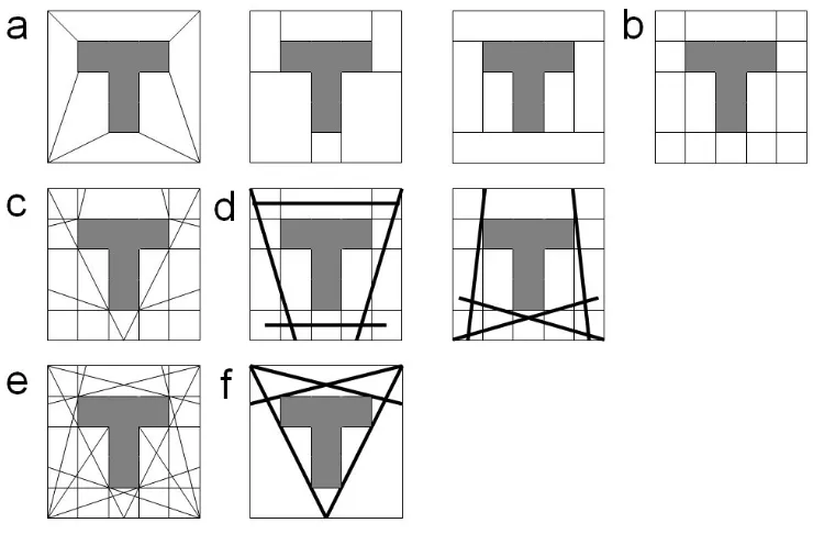
subspaces whose convexity is unique as we illustrate in Figure 1(a). But they suggest that it is possible to generate a larger number of convex spaces which they call an s-partition where a s-partition is made at points of discontinuity which define the edges or faces of the space where there is a change in the number of surfaces which come into view as the partition is crossed. We show this in Figure 1(b). They then extend this criterion by defining e-partitions (of which the s-partition is a subset) which are lines between vertices defining the faces or edges of the form in which other faces or edges gradually or immediately become visible as the lines are crossed. These are extendible diagonals and we show such e-partitions and their e-spaces in Figure 1(c). Details of the actual procedure for their definition are given in the Spatialist software used to generate these (see http://www.arch.gatech.edu/~spatial/) and in the various papers by Peponis et al. (1997, 1998). The advantage of these types of decomposition are that they are unique and informationally stable in the sense that they reflect significant visual (geometric) thresholds which can then be subjected to relational analysis in terms of their topology.
2.2 Generating Axial Lines and Axial Maps
without the axial map being connected in this way, so to avoid such problems, an (arbitrary) criterion of making all axial lines link is imposed. Because a unique set of least, fattest convex spaces cannot be defined, it is thus impossible to automate the construction of an axial map. As the procedure is left to the user, then the biggest problem is controlling for the number of axial lines as this is central to the accessibility values which are subsequently computed and used to index the importance of each line. In Figure 1(d), we present intuitively derived axial maps which cover the s-spaces in Figure 1(b) where it is clear that the second map might be said to cover the space ‘less comprehensively’ than the first although the first has slightly ‘longer lines’. It is problems such as this that this paper seeks to resolve.
The all-line axial map first defined and thence published by Penn et al. (1997) but used extensively by Hillier (1996) in his second book, consists of all possible lines that link vertices defining differences in orientation between faces as well as all extensions of faces to meet other faces, with the added constraint that such lines must pass freely through space which is unobstructed. Peponis et al. (1998) present three different methods. These all begin with the all-lines map illustrated in Figure 1(e) and in each case, they reduce the number of lines in this map while meeting different criteria for covering the convex spaces. One of these methods is particularly straightforward being based on ranking the number of diagonals in the all-lines map with respect to the number of s-partitions that each diagonal crosses. The diagonal with most crossing points becomes the first axial line. This and the associated s-partitions are then removed, the remaining diagonals re-ranked, the largest chosen, the set of diagonals and s-partitions reduced further, and so on until all partitions have been crossed. This method leads to the axial map in Figure 1(f) which is closer to but still somewhat different from the first map in Figure 1(d). These methods show promise but as they depend on the vertex geometry of the original plan or layout, they remain restrictive in terms of where lines can be drawn.
2.3 Viewsheds: Isovists and Isovist Fields
Figure 1: Convex Sets, Partitions, and Axial Lines for the Basic T-Shape
viewpoint or viewshed, in one sense, it is deeply embedded in the theory. All the relational analysis between convex spaces and axial lines from which the importance of these spaces or lines is derived, is based on the notion that what is important is the number of different things that might be seen or accessed from a particular space or line, not the actual distance to these different things. In fact, much of the research just summarized on s- and e-partitions as well as on the all-line map is predicated on the notion that points and lines where viewsheds significantly change are key elements in simplifying the space.
Viewshed analysis has been widely developed in landscape studies and is integral to GIS (Rana, 2002) but there has been very little research on is application to urban areas with one or two notable exceptions. Benedikt (1979), in a pioneering paper on urban viewsheds, adopted the term isovist from Tandy (1967) who had used it to describe landscapes. Until quite recently, Benedikt’s ideas were developed in a somewhat ad hoc way by the space syntax community with the clearest statements in Hillier’s (1996) book, and in the Spatialist software developed by the Peponis group. Recently Turner et al. (2001), Batty (2001), Dalton and Dalton (2001), and Ratti (2002) have all suggested that isovists fields represent an alternative way of simplifying urban and building morphologies using ideas from visibility graphs, agent-based modeling, ray tracing, and image analysis. Software such as Depthmap
from Turner (2001), OmniVista from Dalton and Dalton (2001) and Fathom from Intelligent Space (2002) have appeared which makes the generation of isovist fields automatic. There is a strong implication that the isovist field idea is preferable to the definition of axial maps due to its inherently well defined nature and consistent replicability. Desyllas and Duxbury (2001) go further and suggest that isovist fields represent more appropriate ways of measuring accessibility in urban areas than axial maps because isovist fields provide better correlations with observed movements while the problem of averaging observed density volumes along a line is avoided (Turner and Penn, 1999).
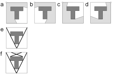
space, somewhat like a diameter. The major difference from space syntax is that isovists are not in general convex spaces although it is possible to define a convex core to each (Hillier, 1996). Although the rest of this paper will be concerned with extracting axial lines from isovists, we must anticipate these to show how they compare to those already described. One method is: first find the isovist with the longest diameter, select this as the first axial line and reduce the space to be considered next by the subtracting the isovist associated with this first line. Then find a viewpoint in the remaining space which generates the next longest line, select this and reduce the space further by subtracting that isovist from the active space. Continue in this manner until all the space has been covered. The set of lines extracted will constitute the axial map. These may not always be connected but their isovists will be, due to the fact that all the space has been systematically considered.
Figure 2: Key Isovists and Related Axial Lines for the Basic T-Shape
2.4 Relational Analysis of Convex Spaces and Axial Lines
Most of the effort in space syntax has not been in generating axial lines or maps but in deriving and interpreting relationships between the lines that comprise such maps through the number of changes of direction or the number of paths between lines defining the spaces comprising the system. In essence, relations between convex spaces can be measured in terms of whether or not common adjacencies exist, or between axial lines in terms of whether or not intersections with other lines exist. If we call the spaces or lines i, j,=1,2,...,N and the number of adjacencies or intersections k,l,=1,2,...,M , the matrix A=[Aik] defines the existence Aik =1 (or
not Aik =0) of adjacencies and intersections k that are associated with spaces or lines
i. The matrix of relations between pairs of spaces or pairs of lines is computed as
∑
= k ik jk
ij A A
R or R =AAT, from which we define the binary matrix L as
. otherwise ,
0 or , , 0 if
1 > ≠ =
= ij ij
ij R i j L
L From the graph implied by this
N t
L L
L t
lj l il t
ij , 1,2,...,
1 1=
∑
=+ with the shortest path between i and j given by the
matrix D t L Lt t N
ij t
ij
ij 1if 0and 0, 1,2,...,
1 > = =
+
= + .
From the shortest path matrix, distances associated with each node (space or line) are computed as sums of indegrees or outdegrees. That is, a typical total distance (or
depth) for a line i is computed as Di =
∑
jDij which is also proportional to theaccessibility or integration of the line. In fact, integration is usually taken as the
inverse −1
i
D and it is these values that are compared to densities or volumes of movement associated with the axial lines. Although most applications of space syntax begin after these integration values have been defined, there are many issues to be clarified concerning the appropriateness of this relational analysis. For example as its well known for any system of relations defined on two sets, there are always dual problems which consist in interpreting relations between one set of elements through the other and vice versa (Batty and Tinkler, 1979). In this case, there is a dual
problem where the matrix of relations is computed from Rˆ =ATA. In the case of
axial maps, the relations would generate accessibilities for the points of intersection, not for the lines themselves. In fact in early studies of urban morphology, Atkin (1974) developed an approach called Q-analysis which sought to examine urban structure in terms of these duals (Atkin, 1974). Such extensions open up an entirely new domain of research in space syntax and we will explore these in a later paper but for now, we will refocus our interest on the extraction of axial lines from isovists and axial maps from isovist fields.
3 Axial Lines from Isovists and Isovist Fields
3.1 Definitions, Properties and Measures
An isovist is defined as the space which can be directly accessed from a specific viewpoint. This might be the space which can be seen by an observer and is often taken (as it is here) as the entire space viewed when the observer moves through 360 0
been restricted to architectural and urban systems at scales where lines of sight are important although in principle, these ideas can also apply to morphologies where sight and vision are not relevant. The focus on scales where vision is relevant, however, is significant because considerable work in space syntax appeals to what and how far one can see as being instrumental in the molding of the urban fabric. With this in mind, an isovist is a non-convex space arrayed around a viewpoint i
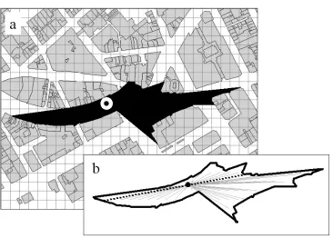
which we illustrate for a small urban streetscape in Figure 3(a). The space is a polygon which in digital applications is approximated by a raster whose points are also illustrated in Figure 3(a). The grid points in this raster are typically other viewpoints for which isovists can also be defined; measures of the shape or what is contained within each isovist are then used to define various isovist fields which are in themselves measures of the morphology of the entire space.
Figure 3: Isovist Resolution and Maximum Diametric Length
viewpoint and measuring the intersection of these rays with the raster points. The method in the ArcView GIS variant used for the public domain code developed here by Rana (see http://www.casa.ucl.ac.uk/spacesyntax/) uses rays but then defines polygons from intersections of the rays with building outlines. A second method used here for the trials in the next section is that developed by Batty (2001) using agent-based technology where agents move along rays, measuring properties of the isovist as they travel. This method developed in StarlogoT is by far the fastest of any to date being implemented on a pseudo parallel processor. The third method developed by Turner (2001), uses the grid points as nodes in a graph which spans the entire space and enables rapid measures of neighborhood and convexity to be calculated in software called Depthmap. The ray and agent tracing is indicated in Figure 3(b) where the rays shown also illustrate all the graph links for the node in question.
The key measure in extracting axial lines as approximations to isovists is based on the diametric length first suggested by Rana and defined as ∆i(jk) =
{
dij +dik}
whereπ θ
θij − ik = and j≠k. The relevant values of this measure are its minimum and maximum given as
{
}
{
d d}
j kd d ik ij ik ij jk i ik ij jk i ≠ = − + = ∆ + = ∆ and where max and min max min π θ
θ . (1)
Hereafter we refer to the maximum diametric length max
i
∆ as the ‘diameter’ of the isovist which we show by the dotted line in Figure 3(b). This defines the longest straight line across the isovist which can be thought of as a maximal spanning distance. Other key measures are the minimum distance and the maximum distance, defined respectively as
{ }
{ }
ijj i
ij j
i d d d
dmin =min and max =max , (2)
with the mean and variance as
2 / 1 2 2( )
− = =
∑
∑
Ω ∈ Ω∈ i j i i
i ij i j i ij i n d d d and n d
d σ . (3)
Means and variances of the diametric lengths are not stated as we will not use them in the subsequent analysis although they are computed by the GIS extension to ArcView
which is described at http://www.casa.ucl.ac.uk/spacesyntax/. A related space exploited by Hillier (1996) associated with any isovist is its convex core and here we note that the minimal convex core is the circle traced out by computing the coordinates around the viewpoint i from ( min)2
i
d
π . We show this core as the larger
When we compute distances, we move the observer m times, incrementing the arc each time by θ =2π /m. The means and variances of these angles are not meaningful but we can compute a weighted mean orientation and variance as
2 / 1 2 2 ) ( ) ( − = =
∑
∑
∑
∑
Ω ∈ Ω ∈ Ω ∈ Ω ∈ i i i i j ij j i ij ij i j ij j ij ij i d d and dd θ θ
θ σ θ
θ . (4)
Area and perimeter computations are straightforward although this requires the end points of each ray to be ordered around the circle of revolution where j=1 is associated with θ, j=2 with 2θ and so on. Defining the radial distance for each ray as riλ, then the area and perimeter are given respectively as
(
) (
)
[
]
1/21
2 1
2 1
2 sin cos
sin 2
1
∑
∑
= + + Ω ∈ − + =
= i i m i i i
i r and p r r r
a i λ λ λ λ λ λ θ θ
θ . (5)
There are several derived statistics useful for measuring the difference between actual and ideal geometric shapes. We define three which all have values of 0 for a straight line shape and 1 for a circle: compactness, Γi, the ratio of average to maximum radial
distance; convexity, Ψi, the ratio of idealized circular to perimeter radius; and
circularity, Θi, the ratio between actual and idealized circular area. A fourth,
centrality, Φi, is a measure of drift or displacement between the centroid of the
isovist and its viewpoint. These measures are defined respectively as
− + − = Φ = Θ = Ψ = Γ
∑
∑
∈Ω ∈Ω 2 / 1 2 2 2 2 / 1max , ,
2 , i i j j i i j j i i i i i i i i i i y n y x n x and d a p a d d i i π π π
. (6)
Isovist fields also have important surface properties which can be exploited to identify various visual thresholds as can be seen in the subsequent examples in this paper as well as in previous published work (Batty, 2001; Turner et al., 2001). These properties have been exploited in landscape analysis (Llobera, 1996; Rana and Morley, 2002) but in this paper, we will simply note that these and their statistics represent an important area for future research.
3.2 Algorithms for Generating Axial Lines
We consider that the axial line associated with an isovist is the maximum diametric
length max
i
∆ defined in equation (1) above. As we have already noted in discussion of axial lines from isovists for the T-shape in Figure 2, this diameter is not associated with a single isovist for there are an infinity of points along its length from which an appropriate isovist can be generated. As axial lines are used to approximate areas, then it is always necessary to select such a line with respect to some areal or other independent measure of an isovist. There must be some way of selecting a unique viewpoint, hence a unique isovist and in this way, the chosen diameter becomes a line uniquely associated with a particular isovist. This is very much in the spirit of space syntax for axial lines are always associated with spaces which they are designed to link and span. Thus their definition from isovist spaces must always relate what is in the space – its area or some other measure – to the way it is approximated by a line. Therefore, the infinity of points on such a line is never at issue and if there are ties to be broken, then this must be accomplished with respect to some other measure of the isovist.
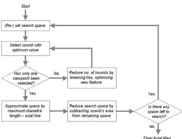
part of a generic algorithm which we describe as follows. The algorithm which we illustrate in Figure 4, works by selecting some attribute or measure of the isovist which is to be optimized. Its begins by selecting the isovist which meets this criterion of optimality and assumes that the space taken by this isovist is dominant. It selects the axial line – the maximum diametric length – associated with this isovist. The next isovist chosen cannot be rooted within the isovist already chosen because that isovist dominates. To make sure that this cannot happen, the space available for searching for the next isovist is reduced by subtracting the first isovist from the entire space. A second isovist which meets the criterion for optimality is then chosen in the reduced space, its axial line selected, and the space further reduced. This process continues until all the space has been covered by isovist selection and at that point, the axial map has been generated. However the axial map is simply an approximation of the dominance ranking of the isovists. The viewpoints and areas of these isovists are equally important to the subsequent analysis of morphology.
The first method which starts with the longest lines essentially is one where the length of line is being optimized. The longest line is chosen and any ties (of which there are many) for isovists associated with this longest line are broken using some other criteria such as largest area. In this way, lines of smaller and smaller length but as long as possible are generated. The second method starts with the isovist associated with the largest area. If there are ties, then these might be broken using the longest line or some other criterion. What this method generates are isovists with smaller and smaller areas. We illustrate the axial lines generated for the T-shape in Figure 2(f) where we begin with the isovists covering the largest areas around the ‘T’ and proceed in the manner just outlined, reducing the space each time. In essence, this method is not dissimilar from that suggested by Hillier and Hanson (1984) for manual definition of axial lines and convex spaces. It is a very strict ranking of lines or spaces where a larger space or longer line completely dominates the selection of the next space or line. In this sense, dominance is a local criterion and the heuristic is locally optimal. Space syntax has never sought to define or aspire to definitions based on global optima for this would involve stating exactly what such optima would entail. This would require setting the problem up as selecting spaces and lines which were as ‘fat’ and as long as possible, respectively, with as few a number of spaces and lines as possible. This would require a definition of ‘fat’ which might be possible from the above measures such as compactness and/or convexity. It would also require formal optimization techniques which take the argument beyond the scope of this paper but it is entirely possible that what space syntax requires are techniques which generate such global optimization. These must await better definitions and explorations in the spirit of the current paper.
simply a summary of spatial orientations. The criterion imposed by Hillier and Hanson (1984) that the map be connected is an arbitrary one. It comes from wanting to imply directional, connective properties to the system that is subsequently used for analysis based on lines of sight which are assumed to be straight.
Second, it is possible to deal with overlapping areas and to deal with isovists which are tied at optimal values. In the longest line approach, we could for example generate all isovists associated with the line, reduce the space accordingly from this mega isovist, and continue in this fashion until all the space is covered. This would give rise to axial lines which were less dense and less connected than for the case where single isovists are identified at each pass of the method. In fact, we have implemented this in our applications to Gassin, and it is of interest to note that this is similar to one of the methods used by Peponis et al. (1998) for generating axial lines which ‘see everything’ but do not necessarily get everywhere. A third problem relates to the appropriateness of the line for indicating space. In the ultimate axial map derived by this method, it is quite possible, indeed usual to see two long lines almost in parallel spanning a space and ultimately intersecting. This is caused by one line being associated with the dominant isovist but that isovist not quite covering a portion of the space that generates it own axial line. At first sight, this might appear that the two lines are of equal dominance in that they are similar in length. However one line is associated with the dominant isovist and although the other line may be as long or longer, its isovist is less dominant than the first and thus has lesser importance in any subsequent analysis. In a sense, to read axial lines associated with this method, the relative importance of the isovist spaces must be considered for there is a strict ranking of lines and spaces according to the criterion used in their selection.
for selection and ranking which are not likely to be correlated. In fact, in many applications of space syntax, there are very strong correlations between the length of axial lines and the subsequent accessibility values produced, for the simple reason that the longer the line, the more likely it is to intersect with other lines. This is an issue that we will touch upon in our examples below but once again, it represents another area of inquiry that is beyond the immediate concern of this paper.
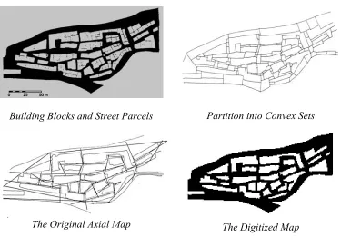
3.3 Comparing Axial Maps: The French Town of Gassin
The small town of Gassin was used by Hillier and Hanson (1984) to originally explain the rudiments of space syntax. It has subsequently been used a test case by Peponis et al. (1998) as well as by Jiang, Claramunt, and Karlqvist (2000) in an alternative reformulation of the theory. The example is manageable in that in the original application only 40 axial lines were defined linking 139 ‘convex’ spaces. In fact, the published data on the maps of the town differ enough to make the definition of axial lines and convex spaces ambiguous and this becomes critical in the methods that we use here which will identify every nook and cranny in the digital representation as being the potential origin of an isovist, hence axial line. Nevertheless, the map that we have taken is sufficiently recognizable and intuitively appreciable as to make this a good test example.
We show the original plan, the convex spaces, and the axial map defined manually and intuitively by Hillier and Hanson (1984) in Figures 5(a), (b), and (c) respectively in comparison to our own scanned map at the resolution used in the StarlogoT
results generated here, the original and the examples developed by Peponis et al. (1998) will solely be in terms of numbers and lengths of axial lines.
Figure 5: Basic Data for the Town of Gassin
Building Blocks and Street Parcels Partition into Convex Sets
The Original Axial Map The Digitized Map
We will first generate a series of isovist fields for Gassin using agent-based methods which walk an agent to all points in the viewshed associated with a given viewpoint. This method generates isovists and isovist fields which are then used to associate different geometric and related measures of properties of viewsheds at each point in
the space (Batty and Jiang, 2000; Batty, 2001). Agents walk 180 in increments of 0 1 0
forwards and backwards from each viewpoint, measuring a series of geometric characteristics from which the set of relevant measures identified earlier in equations (1) to (6) are thence computed. The program for Gassin currently takes about 21 minutes on a McIntosh i-Book (with PowerPC G3 processor running at 366 MHz). In the analysis, we use nine measures, four of which involve the distances
max max
min, , ,and
i i
i
i d d
d ∆ , the area and perimeter measures ai and pi, and three of the
ratio measures – compactness, convexity, and circularity, Γi,Ψi,andΘi. We have
explored in another context. In the professional software based on ArcView, a full set of measures is computed (see http://www.casa.ucl.ac.uk/spacesyntax/).
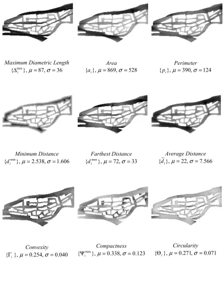
The first stage in generating axial lines is to compute the various isovist fields which are then used for ordering the spaces for which axial lines are used as a summary. The nine fields based on each given measure are shown in Figure 6 where the means and standard deviation of each measure are also shown to provide some comparative basis for the statistics used below. The minimum distance field is the easiest to explain in that it depends entirely on how near the observer is to some edge and the field is largely structured by the width of each street. The largest distances and diameters are
highly correlated (r2 ≈0.835) with the axial structure of the system clearly marked in these fields. In fact, although we will not do so, it appears that these measures could be used directly in the extraction of axial lines although this would depend not on geometric issues which drive the current quest but on image processing techniques (Ratti, 2002). Average distance smoothes the kinds of striations which characterize fields based on minimum and maximum distances but in all these cases, the measures show the existence of visual thresholds particularly at points of discontinuity at points where vistas close or open up.
Figure 6: Isovist Fields for Nine Standard Geometric Measures
Maximum Diametric Length
36 , 87 },
{∆max µ = σ =
i Area 528 , 869 },
{ai µ= σ =
Perimeter
124 ,
390 },
{pi µ= σ =
Minimum Distance 606 . 1 , 538 . 2 },
{ min µ= σ =
i d Farthest Distance 33 , 72 },
{ max µ= σ =
i d Average Distance 566 . 7 , 22 },
{di µ = σ =
Convexity 040 . 0 , 254 . 0 },
{Γi µ = σ =
Compactness 123 . 0 , 338 . 0 },
{Ψmax µ = σ =
i Circularity 071 . 0 , 271 . 0 },
the smaller, shorter streets, and circularity at the edges of the system due to an artifact of the measure itself. As we might expect, there is little association with the pattern of isovists which tend to be non-convex, non-compact, and non-circular in general.
These fields form the measures from which axial lines can be extracted using the algorithm presented earlier and illustrated in Figure 4. In essence, the procedure works with a specific measure for each viewshed or isovist, ordering the isovists according to this measure usually from largest to smallest, starting with the largest and selecting the isovist associated with this as being the most important in the
system. This space is then approximated by the maximum diametric distance max
λ
∆ , the overall space reduced by this isovist and then the next viewpoint and isovist associated with the next largest measure in the remaining space selected. The procedure continues in this way, approximating each subsequent space by its relevant maximum diameter until all space has been covered. We have applied six variants of this algorithm with different measures in each case. The first baseline case adopts the maximum diameter as the measure to optimize and thus the procedure selects space associated with this maximum which is then approximated by the same diameter. The second method is based on area, the third on average distance while the remaining three use the convexity, compactness, and circularity coefficients for the dominance ranking.
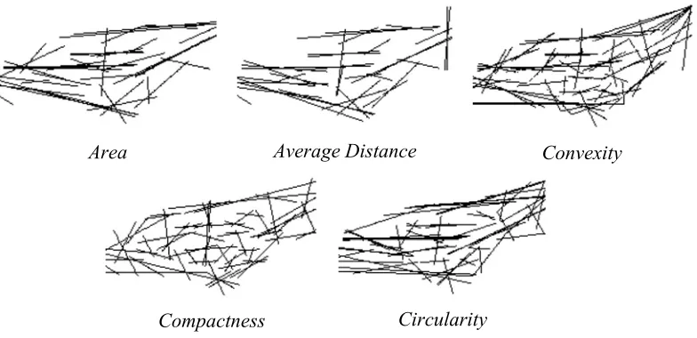
Figure 7: Axial Lines Generated by the Isovist Sorting Algorithm (a) Isovists, Overlaps, Viewsheds, and Axial Maps for the Longest Line Sort
Isovists in Dominance Order Viewpoints of Dominant Isovists
Overlap Count of Dominant Isovists Axial Lines as Maximum Diameters
(b) Axial Maps for the Five Remaining Sorts
Area Average Distance Convexity
Compactness Circularity
different spaces making up a morphology. Notwithstanding the characteristic used to rank importance, the length of the axial line and the area covered by all the associated isovists are basic measures which indicate the efficiency of the application. We only illustrate the axial maps for each of the remaining five applications in Figure 7(b).
It is immediately clear from these results that the rankings based on longest lines, largest areas and largest average distances gives results that are much more efficient than those which depend on the geometric ratios which do not really reflect the linearity of the underlying street system. We illustrate a series of quantitative measures relating to the number and length of lines and areas of associated isovist spaces for each of the six applications in Table 1, where we also contrast these with the more minimal information we have for the Hillier and Hanson (1984) and Peponis et al. (1998) applications. We need to be clear about what is shown here. We will now define the total number of isovists and axial lines generated from each application by
L, the area of the selected isovist by aλ,λ=1,2,...,L and the length of the maximum diametric distance by ∆max,λ=1,2,...,L
λ . In Table 1, we show the number L, the
total line lengths,
∑
λ∆maxλ , the average line length∑
∆ Lλ maxλ , the total area
∑
λ λa ,and the average area
∑
λ λa L. As the selected isovists overlap, we can compare the total area with the actual area of the streetscape (which in this case is 8129 units ofarea). We thus form the ratio
∑
λ λa 8129 which gives the relative duplication of space from such overlaps in comparison to a system where there is no such duplication, as for example in a system divided into mutually exclusive convex spaces as in Figure 5(b).Table 1: A Comparison of Methods for Generating Axial Lines Method No of Axial Lines L Total Line Length
∑
λ∆maxλAverage Line Length
L
∑
λ∆maxλTotal Area Covered
∑
λ λaAverage Area L a
∑
λ λ Area Covered to Total Area 8129∑
λ λaEfficiency Ratio
Ξ
Hillier & Hanson
40 1565 38 nr nr nr nr
Peponis I
13 959 74 nr nr nr nr
Peponis II
37 1635 44 nr nr nr nr
Longest Line
46 3211 70 21500 467 2.645 308
Largest Area
39 2592 66 23225 596 2.857 349
Largest AvDistance
36 2276 63 20628 573 2.538 326
Greatest Convexity
72 3409 47 29971 416 3.687 633
Most Compact
67 2637 39 21929 327 2.698 557
Nearest Circular
60 3768 63 26281 438 3.234 418
minimize the number of these lines as well as their areal linearity. Accordingly we define the measure
∆ = Ξ
∑
∑
λ λ λ λ max aL , (7)
covered smaller at 20667. The ratio methods all generate much larger numbers of lines with the connectivity measure generating twice as many (72) lines as the average distance. The efficiency ratio Ξ bears all this out with the efficiency ranking from the longest line method (best), largest average distance, largest area, greatest circularity, compactness, and connectivity (worst). The key issue here is that the number of axial lines is not in and of itself the most important criterion for this must be matched against their length and the space that they summarize.
3.4 The Statistics of Axial Lines: A Preliminary Analysis
To conclude our analysis of these six applications, we will make a brief foray into the statistical form of the isovist fields and the lines that are generated from the sorting procedures used to partition them into significant viewpoints. An attempt was made by Batty (2001) to initiate such analysis for a range of parameters describing such fields but here we concentrate exclusively on the maximum diametric distance associated with these spaces. There is little doubt that this area is yet another in space syntax analysis which has never been researched and is an essential focus in refining
and extending the theory. The distribution { max
i
∆ } over all 8129 isovists for Gassin is non-normal in that its frequency distribution is bimodal which is a characteristic of linear distances in isovist fields for street systems noted in earlier applications (Batty, 2001). The bimodality essentially classifies isovists into long and short vistas which would appear to be consistent with systems which are dominated by strict hierarchy of streets. The frequency distribution of lengths however is not as useful a plot as the cumulative frequency and the form that we prefer here, much used in scaling analysis, is called the rank-size. This is based on a plot of the distance lengths against their rank
which we show for the set { max
i
∆ } in Figure 8 where we show the frequency,
cumulative frequency and the rank-size which is a reverse plot of the cumulative frequency from largest to smallest distance.
The rank-size is essentially linear with an r2 ≈0.983. There is thus no evidence of
Figure 8: Frequencies and Rank-Size Distributions of Maximum Diametric Lengths
0 F
requ
enc
y
350
0 Maximum Diametric Lengths 158 0% Cu
mulative Frequency
10
0%
0
Diametric Length 1
60
1 Rank of Diametric Length 8129
This is the criterion for scaling which we might expect when we examine the distribution of isovists lengths which form the axial map.
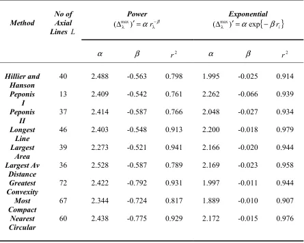
Table 2: Estimation of Power and Exponential Relations for Axial Distances
Power
β
α −
= ′ ∆λ ) rλ
( max
Exponential
{
βri}
α −
= ′
∆ ) exp
( max
λ
Method
No of Axial Lines L
α β r2 α β r2
Hillier and
Hanson 40 2.488 -0.563 0.798 1.995 -0.025 0.914 Peponis
I
13 2.409 -0.542 0.761 2.262 -0.066 0.939
Peponis II
37 2.414 -0.587 0.766 2.048 -0.027 0.934
Longest
Line 46 2.403 -0.548 0.913 2.200 -0.018 0.979 Largest
Area 39 2.273 -0.521 0.941 2.166 -0.020 0.944 Largest Av
Distance 36 2.528 -0.587 0.789 2.169 -0.023 0.958 Greatest
Convexity 72 2.422 -0.792 0.931 1.997 -0.011 0.944 Most
Compact 67 2.344 -0.724 0.817 1.889 -0.010 0.907 Nearest
Circular 60 2.438 -0.775 0.929 2.172 -0.015 0.976
In Figure 9, we have graphed the rank-size relations based on each set { max
λ
∆ } for
each of the six applications of the algorithm. These show a degree of scaling although when presented in logarithm form, they imply something closer to log normality than the classic Pareto power function. In Table 2, we show these relations fitted for two
functions: the traditional power law form ∆ ′=α −β λ
λ ) r
( max and the exponential form
{
βri}
α −
= ′
∆ ) exp
( max
λ where the results are all significant for both models with the
Figure 9: Rank-Size Distribution of Maximum Diametric Lengths
Maximum
Diam
etric Length
Rank of Length
1 Hillier and Hanson 2 Peponis I 3 Peponis II
4 Longest Line 5 Largest Area 6 Largest Average Distance
7 Greatest Convexity 8 Most Compact 9 Nearest Circular
compare the line lengths for the Hillier and Hanson (1984) and Peponis et al. (1998) examples in this table where it is clear too that the axial lines produced by these traditional methods are also scaling. This is good initial evidence that axial lines are scaling due to the process of their selection and the general space syntax assumption that it is essential to identify the importance of spaces according to their area with the largest spaces taking priority.
be compared against diametric length and area to establish these relations. We show these ten sets of relations as scatter plots in Figure 10 with the coefficients of determination alongside. It is clear that there are reasonably strong correlations between line and area from Figures 10(a) and (b) but it is also clear that selecting on the basis of, say, area, does not guarantee that the longest lines are chosen. The same is true for average distance in Figure 10(c) and we also show the relations between this and area which is very strong in 10(d). In this case, average distance basically double counts certain areas of each isovist due to the rotational manner in which cells are accessed and thus this average can only be considered a poor proxy for area. In the case of the ratio coefficients, the strength of relations with line and area are quite weak with the exception of the connectivity index which has a reasonably strong correlation with diametric length. This serves once again to impress the fact that the longest lines and largest areas are not necessarily selected if the optimization is based on some other measure which the isovist captures.
4 An Improved Algorithm: The Full Gassin Application
4.1 Scale and Resolution in Space Syntax
Figure 10: Correlations Between Axial Line Generators, Line Length and Area
Area – Line
679 . 0
2 =
r
Line – Area
658 . 0
2 =
r
Line – Average Distance
628 . 0
2 =
r
Area – Average Distance
902 . 0
2 =
r
Line – Convexity
017 . 0
2 =
r
Area – Convexity
093 . 0
2 =
r
Line – Compactness
084 . 0
2 =
r
Area – Compactness 00 . 0
2 =
r
Line – Circularity 659 . 0
2 =
r
Area – Circularity 397 . 0
2 =
of resolution. In turn this means that the number of axial lines derived traditionally by manual means or by using the algorithm developed here would vary. As more detail is picked up at ever finer scales, the number of axial lines increases.
Analysis of scale and aggregation is central to contemporary spatial analysis. The most comprehensive statement is by Openshaw (1984) who identified crucial changes posed by aggregating scale as the modifiable areal unit problem. In essence, he argued that as the scale of representation changes and if the morphology of the space which is used to classify spatial variation changes too, conventional spatial analysis would yield differing results which, in the extreme, might lead to contradictory inferences at different scales. A variant of this problem in terms of measurement involves the notion of the fractal line in that as the scale becomes finer, more and more detail is picked up, leading to changes in standard measurements such as the length of a line. This has been demonstrated many times, the most famous examples being for coastlines (Mandelbrot, 1967) and political borders (Richardson, 1960).
Table 3: Axial Lines for Gassin at Different Scales
Level of Pixel
Resolution Size of Pixel Space Streetscape Pixels in No of Axial Lines Time for Sorting Algorithm
2 x 2 201 x 201 8129 46 21 minutes
4 x 4 101 x 101 2329 26 4 minutes
8 x 8 51 x 51 737 7 2 minutes
16 x 16 25 x 25 204 2 1.5 minutes
4.2 Axial Lines and Isovist Fields in GIS: The ArcView Extension
We compute and sort the isovists based on the strict hierarchy of maximum diametric lengths using the detailed plan of Gassin shown in Figure 11(a). We have set the parameters – the number of viewpoints, and the incremental angle – at the same levels of resolution as the applications given in the previous section with around 8000
viewpoints and a 1 angle of sweep. However as Figure 11(a) shows, the town plan is 0
at a much higher level of resolution than the previous applications and thus the number of irregular building faces far exceeds those of the digitized plan in Figure 5(d). Thus one would expect there to be more isovists generated through the sorting procedure as more detail is being picked up. This is borne out in the fact that the number of isovists, thence axial lines selected is 56, some 20 percent more than the cruder digitization but consistent with the relation implied in Table 3. These are shown in Figure 11(b). However what this application suggests is that the number of axial lines would vary much less when the density of viewpoints changes than in the case where the level of resolution of the building outlines and streetscape change.
There are many advantages to implementing such algorithms within well-developed standard software such as ArcView which is extremely modest in cost. In particular, the many extensions that can be used to visualize and compute spatial metrics for maps and layouts help extend the analysis. What we are able to do here is to visualize the way isovists overlap with one another much more easily than we did in Figure 7 by invoking the 3d-Analyst extension. In Figure 12, we show two perspective views of the overlap where we have colored the isovists according to the scale of their dominance and ordered them in 3-d from top to bottom. This shows immediately how axial lines are a very weak way of visualizing this kind of spatial complexity. It also shows that the sorting algorithm we use always leads to isovists which are connected through their overlaps because the original streetscape space is connected.
Figure 12: 2-d and 3-d Views of the Dominance Hierarchy of Overlapping Isovists
5 Conclusions: Next Steps
and ensure that these lines connect, all coming under scrutiny in terms of the best way of representing urban morphology. Moreover, this representation must be tied much more strongly to behavioral issues, to the nature of economic activities in cities which is the core of urban geography, and to ways in which people interact through various modes of transport.
Space syntax needs to be considered as one version of the generic problem of spatial representation which involves simplification of geometric form to reflect more parsimonious ways of understanding the importance of different spaces and the way they are related. In this sense, the axial line is probably not the appropriate unit of analysis but something more basic such as the parcel or even some fine level grid should be explored. In short, space syntax needs to embrace and relate to other approaches to urban morphology such as shape grammars, Q-analysis, cellular systems, fractal representations and so on. This is the wider and longer term agenda. In the shorter term, the strictures posed by summarizing space by straight lines need to be explored further, and this in turn raise questions as to the purpose of defining such lines when simpler and more obvious ways of relating the spaces that they summarize are readily available.
With respect to the actual methods presented here, there is much work to do. The basic algorithm we have developed sorts isovists according to a very strict dominance ranking. We need to relax this in the manner that we noted in our final example where the larger isovist envelope based on the longest axial line was constructed and then used as a basis for ranking. We also intend to explore ways in which isovists might be used as seeds in some evolutionary solution to generating spatial subdivisions which meet a variety of criteria, thus synthesizing bottom-up criteria with top-down. This will lead us to pose the partition problem is a rather different way, taking us to global rather than local optimization.
with varying terrain (because the terrain of Gassin was not published in the original application), it would be a simple matter to add height to the raster and to truncate the ray tracing when distant areas disappear from sight. True extensions to deal with 3-d environments are on the horizon but once again, real progress can only be made if the basic space syntax problem is reformulated.
In short, a major research program is required which must be part of our wider quest to develop better ways of representing urban morphology so we can understand the ways building and townscapes evolve through organic growth and change as well as through design. We are already examining a whole series of extensions to the problem of isovist representation and sorting using the methods that that we have presented here while we are also working on ways of representing relations between spaces using standard ideas of graph theory which are in use in other areas. These, we hope, will provide us with firmer foundations for space syntax in particular, and the study of urban and architectural morphology in general.
6 References
Atkin, R. H. (1974) Mathematical Structure in Human Affairs, Heinemann
Educational Books, London.
Batty, M. (2001) Exploring isovist fields: space and shape in architectural and urban morphology, Environment and Planning B, 28, 123-150.
Batty, M., and Jiang, B. (2000) Multi-agent simulation: computational space-time dynamics in GIS, in P. Atkinson and D. Martin (Editors) Innovations in GIS VII: GIS and Geocomputation, Taylor and Francis, London, 55-71.
Batty, M., and Tinkler, K. J. (1979) Symmetric structure in spatial and social processes, Environment and Planning B, 6, 3-27.
Benedikt, M. L. (1979) To take hold of space: isovists and isovist fields,
Environment and Planning B, 6, 47-65.
Dalton, R, C. and Dalton, N. (2001) OmniVista: an application of isovist field and path analysis, Proceedings, Third International Symposium on Space Syntax
Desyllas, J. and Duxbury, E. (2001) Axial maps and visibility analysis: a comparison of their methodology and use in models of urban pedestrian movement, Proceedings, Third International Symposium on Space Syntax (Atlanta 2001), 27.1-27.13.
Hillier, B. (1996) Space is the Machine: A Configurational Theory of
Architecture, Cambridge University Press, Cambridge, UK.
Hillier, B., and Hanson, J. (1984) The Social Logic of Space, Cambridge University Press, Cambridge, UK.
Intelligent Space (2002) FATHOM: visibility graph analysis software, details available from http://www.intelligentspace.com/tech/fathom.htm accessed 6/8/2002 and from Intelligent Space Partnership, 68 Great Eastern Street, London, EC2A 3JT, UK.
Jiang, B., Claramunt, C. and Karlqvist, B. (2000) An integration of space syntax into GIS for modeling urban spaces, JAG, 2, 161-171.
Llobera, M. (1996) Exploring the topography of mind: GIS, social space and archaeology, Antiquity, 70, 612-622.
Mandelbrot, B. B. (1967) How long is the coast of Britain? Statistical self similarity and fractal dimension, Science, 155, 636-638.
Openshaw, S. (1984) The Modifiable Areal Unit Problem, Concepts and
Techniques in Modern Geography, 38, Geobooks, Norwich, UK.
O’Rourke, J. (1987) Art Gallery Theorems and Algorithms, Oxford University Press, New York.
Penn, A., Conroy, R., Dalton, N., Dekker, L., Mottram, C., and Turner, A. (1997) Intelligent architecture: new tools for three dimensional analysis of space and built form, Proceedings, First International Symposium on Space Syntax (London 1997), 30.1-30.19.
Peponis, J., Wineman, J., Rashid, M., Kim, S. H., and Bafna, S. (1997) On the description of shape and spatial configuration inside buildings: convex partitions and their local properties, Environment and Planning B, 24, 761-781.
Peponis, J., Wineman, J., Bafna, S., Rashid, M., and Kim, S. H. (1998) On the generation of linear representations of spatial configuration, Environment and Planning B, 25, 559-576.
Rana, S. (2002) Fast Viewshed computation using topographic features, Proceedings,
GISRUK 2002 (Sheffield), 16-21.
Rana, S., and Morley, J. (2002) Surface Networks, Working Paper 43, Centre for Advanced Spatial Analysis, University College, London, accessed 6/8/2002 at
Ratti, C. (2002) Urban Analysis for Environmental Prediction, PhD Dissertation, University of Cambridge, Department of Architecture, Cambridge, UK.
Richardson, L. F. (1961) The problem of contiguity: an appendix to ‘The Statistics of Deadly Quarrels’, General Systems Yearbook, 6, 139-187.
Tandy, C. R. V. (1967) The isovist method of landscape survey, in H. C. Murray (Editor) Symposium on Methods of Landscape Analysis, Landscape Research Group, London, 9-10.
Turner, A. (2001) Depthmap: a program to perform visibility graph analysis,
Proceedings, Third International Symposium on Space Syntax (Atlanta 2001), 31.1- 31.9.
Turner, A. and Penn, A. (1999) Making isovists syntactic: isovist integration analysis,
Proceedings, Second International Symposium on Space Syntax (Brazilia 1999), accessed 6/8/2002 at http://www.spacesyntax.com/ss2abstracts/turner.html
Turner, A., Doxa, M., O’Sullivan, D., and Penn, A. (2001) From isovists to visibility graphs: a methodology for the analysis of architectural space, Environment and Planning B, 28, 103 – 121.