a
Corresponding author: [email protected]
Boiling heat transfer on fins – experimental and numerical procedure
T. Orzechowski1,a, A. Tyburczyk1 1
Environmental Engineering Dep., Heat Engineering Div., Kielce University of Technology, Al. Tysiąclecia PP 7, 25-314 Kielce, Poland
Abstract.The paper presents the research methodology, the test facility and the results of investigations into non-isothermal surfaces in water boiling at atmospheric pressure, together with a discussion of errors. The investigations were conducted for two aluminium samples with technically smooth surfaces and thickness of 4 mm and 10 mm, respectively. For the sample of lower thickness, on the basis of the surface temperature distribution measured with an infrared camera, the local heat flux and the heat transfer coefficient were determined and shown in the form of a boiling curve. For the thicker sample, for which 1-D model cannot be used, numerical calculations were conducted. They resulted in obtaining the values of the local heat flux on the surface the invisible to the infrared, camera i.e. on the side on which the boiling of the medium proceeds.
1 Introduction
In the recent years, the heat transfer processes have been thoroughly investigated. The interest in those phenomena results from the possibility of carrying away heat fluxes of substantial density. Such solutions allow the construction of more efficient devices and, consequently, a reduction in the materials costs of heat exchangers and in energy consumption in industrial processes.
The tasks mentioned above provide a stimulus to numerous research activities aimed at increasing the efficiency of devices in which heat transfer processes occur. In order to reach the goal, it is necessary to obtain the highest possible values of heat transfer coefficient, i.e. the largest possible heat flux for a small temperature difference between the heating surface and the fluid in contact with it. That can be achieved due to the change of phase which accompanies a boiling process.
Boiling heat transfer is affected by many factors related to the conditions under which the process proceeds, and also the parameters of the surface material and geometry. Those factors occur at the same time and interact. Heat transfer coefficient is considerably affected by, among others, saturation pressure, thermal and physical properties of the working fluid, and also thermal and physical properties of the heater, e.g. the material heat conduction coefficient, wettability, external dimensions, and surface morphology or spatial orientation [1].
For example, Das et al. [2] tested several structured surfaces in order to assess their impact on the process of heat transfer enhancement. Distilled water under atmospheric pressure was used as the test fluid. The surfaces used in the experiment had many parallel or
orthogonally intersecting tunnels. The effect of design parameters, including tunnel inclination and different cavity structure at the tunnel base, on the boiling heat transfer was investigated. Three different structures, namely with circular, rectangular and rounded grooves at the tunnel end were used. The heat flux varied in the range from 0 to 250 kW m-2. Experimental results show that tunnels inclined at an angle 60o to the horizontal provide better enhancement when compared with straight vertical tunnels. The use of tunnels inside the surface contributes to boiling heat transfer enhancement, additionally, as regards different base geometries, the circular pocket facilitates the process even further. The highest increase in the critical heat flux (CHF) was obtained for the surface with sloping tunnels and a circular base.
Kang [3] gave results of investigations into the effect of the heating surface roughness and spatial orientation for water boiling on stainless pipes at ambient pressure. The inclination angle ranged from 0o (horizontal surface), 45o, 90o (vertical surface) and the average roughness was 60.9 nm and 15.1 nm. Pipes were 9.7 mm, 19.05 mm and 25.4 mm in diameter. It is observed that increased roughness facilitates boiling heat transfer. That is related to the density of nucleation centres, from which bubbles depart. The greater is the inclination, the more visible is the impact.
El-Genk and Bostanci [4] presented the results of investigations into the effect of the heating surface inclination on heat transfer. The experiment was conducted on 10 x 10mm flat copper surface, and HFE-7100 was a working fluid. The surface inclination ranged 0o (horizontal surface), 30o, 60o, 90o (vertical surface), 120o, 150o, and 180o. For the inclination that does not
This is an Open Access article distributed under the terms of the Creative Commons Attribution License 2.0, which permits unrestricted use, distribution, and reproduction in any medium, provided the original work is properly cited.
C
exceed 90o and the superheat greater than 20 K, the heat flux density decreases with an increase in inclination, which the authors attribute to the accumulation of bubbles near the heating surface. The heat flux density, however, grows with an increase in the inclination angle for small superheats, which results from enhanced mixing within the wall-adjacent layer. For the inclination greater than 90o and the superheat higher than 13 K, a drop in the heat flux density is also observed to accompany inclination increase.
Priarone [5] conducted an experiment to examine the effect of a smooth copper surface orientation on the boiling process. The investigations were performed for two dielectric fluids: FC-72 and HFE-7100 under ambient pressure. For both fluids, the inclination angle of the copper surface to the horizontal plane was changed at regular intervals and ranged from 0o (upper surface) to 175o. The results obtained in the experiment confirmed some of the effects of heater orientation on heat transfer coefficients, described in the literature. In the range of low heat fluxes, the heat transfer coefficient increases significantly with the angle of the surface orientation, while for higher heat flux values, the orientation effect is visible only for angles greater than 90o, and then the heat transfer coefficient decreases with an increasing angle. The CHF decreases slightly at an angle of orientation in the range of 0o to 90o, but CHF rapidly decreases for angles up to 180o. CHF values obtained for the two fluids and for different angles, normalized to the maximum value of 0o, showed good congruence with the correlations given in the literature. Heat transfer coefficients and CHF for HFE-7100 were higher than in the case of FC-72 liquid.
Having analysed the impact of roughness, Ribatski and Saiz Jabardo [6] stated that an increase in the heat transfer rate that accompanies increased roughness results from the growing density of the active nucleation centres which generate vapour on the heating surface. Consequently, heat transfer on the surface that has greater roughness is more intensive, which is confirmed by the results obtained by the authors. They were also concerned with the impact the heating surface material has on heat transfer. In the authors’ opinion, that depends on the working fluid used. For R-11 fluid and 0.16 μm roughness, the best results were achieved for a brass surface. Yet for R-12, boiling curves for brass and copper almost coincide. Generally, for the working media tested, the greatest densities of the rejected heats fluxes were observed for brass surfaces, then for copper ones, whereas the smallest densities were found for stainless steel.
In [7] Wen et al. presented a comparative study concerning the impact of nanofluids on heat transfer processes. The experiment was performed with two specially designed surfaces. Detailed description of the surface before and after the boiling process shows that the change in the geometry of the heating surface is mostly responsible for many contradictory results described in the literature. The improvement or deterioration of boiling heat transfer when using nanofluids depends on various surface modifications, the
size of particles suspended in the liquid, the heating surface geometry, and their interactions.
Wu and colleagues [8] performed investigations to analyze the process of the formation of nucleation centres in the boiling liquid and to measure the critical heat flux (CHF) on the surface modified with titanium oxide (TiO2). In the experiment, 1 cm2 of the copper surface coated with a TiO2 layer, 1 ȝm in thickness, was heated. Water and highly wetting liquid, FC-72, were used in the process. The results were compared with those for a smooth surface. The comparison showed that TiO2-coated surface increased CHF by 50.4% for water and 38.2% for FC-72. Thus, it was demonstrated that an increase in heat transfer depends on the degree of wettability. The data confirmed that the hydrophilicity of TiO2-coated surface can also alter the mechanism of boiling heat transfer.
Yu and Lu [9] conducted an experiment on copper surfaces with a rectangular fin array, immersed in the saturated fluid FC-72. They studied the effect of geometrical parameters (spacing and length of the fins) on the performance of the boiling process. The surfaces of the test block, made of copper, had a base area of 10 mm x 10 mm. The fins, of four lengths (0.5 mm, 1.0 mm, 2.0 mm and 4.0 mm) were arranged in three spacing patterns, namely 0.5 mm, 1.0 mm and 2.0 mm apart. The investigations were conducted at atmospheric pressure. A flat surface was assumed to be a reference surface, with which finned surfaces were compared. The test results showed that more closely arranged and bigger fins provide greater resistance to flow. Further, when the heat flux was close to the critical one (CHF), numerous vapour bubbles were formed, which departed from the surface, causing the drying of the plate centre. The results also showed that the heat transfer coefficient decreased rapidly when the spacing of the fins was reduced or the fin length increased. The maximum value of CHF on the base surface was 9.8 · 105 W m-2, which was found for the test surface with 0.5 mm spacing and 4.0 mm length of the fins. This value was five times higher than that for the surface without fins.
All the factors discussed above contribute to discrepancies in the results of experimental investigations quoted by different authors. Hobler [10], for instance, analysed twelve different correlation equations that describe water boiling on smooth surfaces at ambient pressure. The values of heat flux densities, calculated with those correlations, demonstrate considerable differences. That can be explained by different conditions, under which measurements were taken, and also by the condition of the surface under investigation. Furthermore, a satisfactory model of the physical process of boiling is still not available. Such a model would provide a basis to predict the operation of heat exchangers, which is discussed in detail by CieĞliĔski [11].
The present paper aims to utilise experimental investigations, conducted on individual basis, to design components of heat exchanger systems, and, on the basis of the measurement of the temperature distribution in a one-dimensional model, to transfer it to a two-dimensional model.
2 Test facility
Investigations were conducted at the test facility, specially arranged for the task. The diagram of the facility is presented in figure 1.
Figure 1. Diagram of the test facility for non-isothermal
samples 1 – the examined element, 2 – the thermovision camera, 3 – the auxiliary heater, 4 – the separation system with the control of supplied electric power, 5 – the main heater system with the electric power measurement, 6 – the main heater, 7 – the liquid supply and condensate recovery system, 8 – temperature measurement and control system.
A smooth fin, 4 mm in thickness and approx. 70 mm in length, was a main component of the test facility. It was fixed between two bakelite plates, which at the same time provided a casing of the vessel filled with the liquid. The test facility was equipped with two independent heating systems. The main heating element, whose power was controlled with an autotransformer, was located at the fin base. The auxiliary heating system, made of spirally coiled resistance wire, was positioned on the bottom of the vessel. A constant supply of the electric power to the auxiliary system was maintained throughout all measurement series. The task of the auxiliary system was to sustain the boiling process in the whole volume of the liquid. Supplying power to the auxiliary system was preceded by a measurement intended to examine the effect produced by the power supply on the results of investigations. Within the whole range of the power supply, no such effect was observed. The test facility was equipped with a cooling and condensate recovery system. Vapours of the boiling liquid condensed in the system of two tap water-cooled condensers, and then flowed, by gravity, into the vessel.
Figure 2 presents the element view, where one side of the tested fin is in contact with the boiling liquid, and the other (the outer one), with the atmosphere.
Measurements of the surface temperature distribution on the fin external side were taken with the VarioCAM hr thermovision camera manufactured by a German
company Jenoptik. The camera was equipped with uncooled bolometric matrix providing 640 x 480 pixel format. The device was designed to operate within a long-wave range of infrared radiation (7.5 ÷ 14 µm). The investigations were conducted using a standard 30 x 230 lens. In order to heighten the accuracy and repeatability of measurements, the surface being observed was evenly covered with a black paint. In separate calibration tests, emission properties of the paint were determined for the camera operation range.
Figure 2. Simplified diagram of the test facility: 1 - fin, 2 -
heating system with electric power measurement, 3 - the main heater, 4 – infrared camera 5 – acquisition and image processing system.
Priori to testing, calibration studies of THV-camera were conducted to determine to emissivity of the surface where the thermal field should have been measured. With this the exact temperature could be set [13].
3
Research methodology
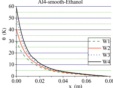
The experimental set-up of the facility makes it possible to work on the assumption that the phenomenon is one-dimensional, that is to assume that the temperature change along the fin thickness is so small that it can be disregarded. The assumption is correct for numbers Bi < 0.1 [14]. Consequently, the results of investigations come in a form of one-dimensional temperature distribution over the fin length, along its axis. Exemplary measurement results for a smooth surface aluminium specimen are shown in figure 3.
0.00 0.02 0.04 0.06 0.08
0 10 20 30 40 50 60
θ
(Κ
)
x (m)
W1 W2 W3 W4 Al4-smooth-Ethanol
Figure 3. Axial temperature distribution for a 4 mm thick
Results presented in figure 3 were obtained for four different heating powers supplied to the fin base.
Using a thermovision camera, it possible to obtain a very large number of measurement points. That, in turn, makes it possible to apply numerical differentiation methods with simultaneous smoothing. In this way, the temperature derivative over the fin length is determined. In accordance with Fourier Law, it is proportional to the amount of transposed heat.
Those data can be presented in a different system of coordinates. It is characteristic that the results for all measurement powers are located along a single curve. That makes it possible to approximate the curve with an arbitrary function [14]. Generally, it is the most convenient to apply polynomial approximation, which is presented in figure 4.
0 10 20 30 40 50 60
0.0 5.0x10⁶ 1.0x10⁷ 1.5x10⁷ 2.0x10⁷ 2.5x10⁷ 3.0x10⁷ 3.5x10⁷
Al4-smooth-Ethanol
W1 W2 W3 W4
polynomial fit
(δ
θ/
δ
x)
2
(
K
2 m
-2 )
θ (K)
Figure 4. Dependence of the gradient square of the superheat
for a smooth aluminium specimen.
On that basis, it is possible to determine a boiling curve, which for the element under consideration, is presented in figure 5.
1 10 100
102 103 104 105
106 Al4-smooth-Ethanol q poly 6
α poly 6 q calculated
α calculated
α (
Wm
-2 K
-1 )
q
(Wm
-2 )
θ (Κ)
Figure 5. Boiling curves for a smooth aluminium sample, 4 mm
in width.
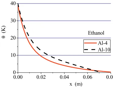
Following the procedure described above, and under identical conditions, the tests were conducted for an aluminium sample, 10 mm in thickness. Axial temperature distribution for different thickness of smooth aluminium fins are presented in figures 6 and 7. All measurement data start from the same temperature at the base. At equal superheat at the base, temperature distributions measured with infrared camera for samples,
4 mm and 10 mm in thickness, differ significantly from each other, as, for the sake of example, was shown in figure 8.
0.00 0.02 0.04 0.06 0.08
0 10 20 30 40
θ
(
K
)
x (m) W2 W3 W4
Averaged Curve Al4 -smooth-Ethanol
Figure 6. Exemplary axial temperature distribution for 4 mm
thick aluminium fin of smooth surface.
0.00 0.02 0.04 0.06
0 10 20 30 40
W1 W2 W3 W4
Averaged Curve
θ
(
K
)
x (m) Al 10-smooth-Ethanol
Figure 7. Exemplary axial temperature distribution for 10 mm
thick smooth aluminium fin.
0.00 0.02 0.04 0.06 0.08
0 10 20 30 40
θ
(
K
)
x (m)
Al-4 Al-10 Ethanol
Figure 8. Exemplary axial temperature distribution for 4 and 10
mm thick fin.
different amount of heat carried away from its surface. At the same time, a relatively large sample thickness does not allow the use of the 1-D analysis discussed above. In that case, the task must therefore be solved numerically.
4
Numerical methods
The correctness of the simplifying assumptions made for the adopted methodology of determining a boiling curve was checked by comparing the results obtained experimentally with numerical calculations.
In order to model the system, the energy balance method was used, where the finite-difference equation for a node is obtained by applying conservation of energy to a control volume about the nodal region.
The cross section of the element under consideration is rectangular in shape. Four boundary conditions are specified for the rectangle. They result from the system geometry and the test facility construction, which was described in Section 2:
• for x = 0, the temperature at the fin base is constant and it is known,
• for y = 0, the temperature is given on the element surface (figure 3) for the power, assumed for calculations, supplied to the main heater,
• for x = L, i.e. at the fin tip, the superheat is close to zero, whereas its derivative also equals zero because of the length of the examined element,
• on the side in contact with the boiling liquid y = h, the density of the heat flux carried away depends on the superheat and the heat transfer coefficient Į of the functional dependence obtained with the 1-D analysis.
In the last condition, a non-linearity is found that is connected with Į coefficient, which is a function of the superheat, in the form of usually sixth- or fifth-degree polynomial. Therefore, a solution to the problem has to be sought numerically. Exemplary energy balances for two internal and one boundary nodes are presented, in the form of a diagram, in figure 9.
Figure 9. Exemplary balanced nodes.
On the line x = const., those have the following form: • energy balance equation for point Ti,j
1 , 2 1 , , 2 , 1 , ,
1 2 ( 2 )
− + + − ¸¸¹ · ¨¨© § Δ Δ − = + − ¸¸¹ · ¨¨© § Δ Δ + + − j i j i j i j i j i j i T y x T T y x T T T (1)
• energy balance equation for point Ti,j+1
0 ) 2 ( 2 2 , 1 , , 2 1 , 1 1 , 1 , 1 = + − ¸¸¹ · ¨¨© § Δ Δ + + − + + + + + + − j i j i j i j i j i j i T T T y x T T T (2)
• energy balance equation for point Ti,j+2
0 2 ) ( 2 2 2 , 2 2 , 1 , 2 2 , 1 2 , 2 , 1 = Δ ¸¸¹ · ¨¨© § Δ Δ − − ¸¸¹ · ¨¨© § Δ Δ + + − + + + + + + + − j i j i j i j i j i j i T y y x T T y x T T T λ
α (3)
For the whole area, the procedure yields a system of equations, the number of which equals the number of unknowns. Because of the non-linearity mentioned before, the problem is solved using the iterative method of successive approximations. In order to determine the first approximation, the known, i.e. measured on the boundary that can be seen, temperature distribution is used. In this way a system of linear equations is obtained, which has the following form:
B
AT= (4)
and the solution to which can be symbolically written as:
B
A
T
=
−1(5)
5 Method validation
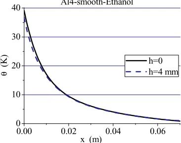
Due to the different temperature distribution on the fin side visible to the THV camera, for thicker samples, an assumption on one-dimensional conductive state cannot be made. In the case of concern, the calculations should be made on the basis of a two-dimensional model. A boundary condition for the thermal imager is necessary. It will take the form of the condition of the third kind, which corresponds to the occurrence of convection cooling. Because of the identical operating conditions of the two fins, the pre-determined dependence for a thin fin can be used for calculations.
0.00 0.02 0.04 0.06
0 10 20 30 40 Al4-smooth-Ethanol θ (K)
x (m)
h=0 h=4 mm
Figure 10. Temperature distribution along the fin length for the
surface on the side of the camera (y = 0) and for the surface on the side of the fluid (y = 4 mm).
was determined along the fin length for the camera-side surface (y = 0), and for the surface side in contact with the fluid (y = 4 mm). Then, on the basis of experimental and numerical data, a boiling curve was plotted, as shown in figure 11.
0 1x10⁵
2x10⁵ 3x10⁵ 4x10⁵ 0
2500 5000 7500
10000 Al4-smooth-Ethanol
experiment poly 6 numerical calculation
α
(
W
m
-2 K
-1 )
q (Wm-2)
Figure 11. Dependence of the heat transfer coefficient on the
heat flux density, obtained numerically and experimentally.
The curves presented in figure 11 almost coincide, indicating the correctness of the calculation algorithm used in the study.
6 Numerical calculations
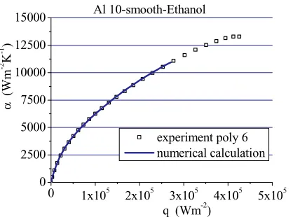
In the same manner as for the thin fin, temperature distribution along the fin length was determined numerically for the other test sample with a thickness of 10 mm. The results are shown in figure 12 and 13. Compared with the previous sample, the temperature difference at the invisible edge is more clearly marked than at the visible one.
0.00 0.02 0.04 0.06
0 10 20 30 40
θ
(K
)
x (m)
h=0 h=10 mm Al 10-smooth-Ethanol
Figure 12. Temperature distribution along the fin length for the
surface on the side of the camera (y = 0), and for the surface on the side of the fluid (y = 10 mm).
0 1x10⁵
2x10⁵ 3x10⁵ 4x10⁵ 5x10⁵ 0
2500 5000 7500 10000 12500
15000 Al 10-smooth-Ethanol
experiment poly 6 numerical calculation
α
(Wm
-2 K
-1 )
q (Wm-2)
Figure 13. Dependence of the heat transfer coefficient on the
heat flux density, obtained numerically and experimentally.
Figure 8 shows the amount of dissipated heat for the thin and thick fins. These values were determined for the visible surface starting at the same temperature value at the base, in accordance with the formula:
¦
³
≅
¦
Δ
=
Δ
=
i i L
i i
fin
qPdx
q
P
x
P
x
q
Q
0(6)
34
.
1
3561907.69
4759822.84
4 10
4
10
=
=
=
¦
¦
− −
− −
i i
Al fin
Al fin
Al Al
q
q
Q
Q
(7)
where: P element perimeter, m.
Calculations proved that the fin of the thickness of 10 mm carries away 34% more heat than the sample 4 mm in thickness.
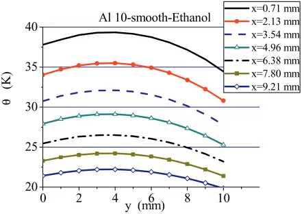
Figures 14 and 15 presents the distribution of temperature on the visible side of the fin along its height (h = 12 mm).
0 1 2 3 4
15 20 25 30 35 40
θ
(K)
y (mm)
x=0.79 mm x=2.13 mm x=3.54 mm x=4.96 mm x=6.38 mm x=7.80 mm x=9.21 mm
Al 4-smooth-Ethanol
Figure 14. The temperature distribution inside the 4 mm fin for
0 2 4 6 8 10 20
25 30 35 40
θ
(K
)
y (mm)
Al 10-smooth-Ethanol x=0.71 mm x=2.13 mm
x=3.54 mm x=4.96 mm x=6.38 mm x=7.80 mm x=9.21 mm
Figure 15. The temperature distribution inside the 10 mm fin
for exempary sections at x = const.
7 Conclusions
The investigations involved a long (approx. 70 mm) aluminium fins, 4 and 10 mm in thickness. The measurements yielded the temperature distribution on the surface viewed by a thermovision camera. The temperature distribution is shown in figures 3 and 7 (lines for y = 0). The opposite surface, on which heat transfer occurs, is not seen by the thermovision camera. The reason for that are poor transmission properties of the fluid in the spectral range of the device.
On the bases of the numerical data he total heat rate loss from visible (from the camera side) and invisible (from the liquid) surfaces can be calculated. The heat received by the atmosphere with respect to the heat received by the ethanol is very small and is only 3.5% of the loss to the ethanol. This indicates an obvious possibility to neglect the cooling of the atmosphere side surface.
The results of experimental investigations and numerical calculations are presented in figures 10, 11, 12, 13, 14 and 15. A small change in temperature distributions between the fin external and internal surface (figures 10 and 12) results from a good thermal conductivity of the material of the fin, which is relatively small in thickness. As a result, measured and numerically calculated values of heat transfer coefficient demonstrate good congruence, which indicates a correct selection of measurement methods and a cogent analysis of the experimental results. It should be emphasised that the experimental results can be successfully applied while designing elements of heat exchange systems manufactured with the same technology and operating under similar conditions, which have different geometry, e.g. are different in thickness.
References
1. I.L. Pioro, W. Rohsenow, S.S. Doerffer, Int. J. Heat Mass Tran., 47 (2004)
2. A.K. Das, P.K. Das, P. Saha, Appl. Therm. Eng., 29 (2009)
3. M.G. Kang, Int. J. Heat Mass Tran., 43 (2000)
4. M.S. El-Genk, H. Bostanci, Int. J. Heat Mass Tran., 46 (2003)
5. A. Priarone, Int. J. Therm. Sci., 44 (2005)
6. G. Ribatski, J.M. Saiz Jabardo, Int. J. Heat Mass Tran., 46 (2003)
7. D. Wen, M. Corr, X. Hu, G. Lin, Int. J. Therm. Sci., 50 (2011)
8. W. Wu, H. Bostanci, L.C. Chow, Y. Hong, M. Sua, J.P. Kizito, Int. J. Heat Mass Tran., 53 (2010) 9. C.K. Yu, D.C. Lu, Int. J. Heat Mass Tran., 50
(2007)
10. T. Hobler, Heat transfer and heat exchangers. WNT, Warszawa, in Polish (1986)
11. P.R. Dominiczak, J.T. CieĞliĔski, Exp. Therm. Fluid Sci. 33, 1 (2008)
12. T. Orzechowski, Boiling heat transfer on fins with structural microcoverings, Kielce, in Polish (2003)
13. T. Kruczek, W. Adamczyk, R.A. Białecki, Int. J. of Thermophys. 34, 3 (2013)
14. F.P. Incropera, et al., Fundamentals and Heat and Mass Transfer, John Wiley & Sons, (2007)