Grey Wolf Optimization for Economic Load
Dispatch with Valve-Point Effects
Fuazen1, Hardiansyah2
Department of Mechanical Engineering, Universitas Muhammadiyah Pontianak, Indonesia1
Department of Electrical Engineering, University of Tanjungpura, Indonesia2
ABSTRACT:Grey Wolf Optimization (GWO) is a new meta-heuristic inspired by grey wolves. The leadership hierarchy and hunting mechanism of the grey wolves is mimicked in GWO. In this paper, GWO is proposed to solve the economic load dispatch (ELD) problem with valve-point effects. To demonstrate the effectiveness of the proposed approach, the numerical studies have been performed for twostandard test systems, i.e. six andfifteen generating unit systems, respectively. The results show that performance of the proposed approach reveal the efficiently and robustness when compared results of other optimization algorithms reported in literature.
KEYWORDS:Grey wolf optimization, economic load dispatch, non-smooth cost functions, valve-point effects.
I.INTRODUCTION
Electrical power system plays a pivotal role in the modern wold to satisfy various needs.Most of power system optimization problems including economic load dispatch (ELD) which have complex and nonlinear characteristics with heavy equality and inequality constraints. The objective of the ELD of electric power generation is to schedule the committed generating unit outputs so as to meet the required load demand at minimum operating cost while satisfying all unit and system equality and inequality constraints. Several classical optimization techniques such as lambda iteration method, gradient method, Newton’s method, linear programming, Interior point method and dynamic programming have been used to solve the basic economic dispatch problem [1]. These mathematical methods require incremental or marginal fuel cost curves which should be monotonically increasing to find global optimal solution. In reality, however, the input-output characteristics of generating units are non-convex due to valve-point loadings and multi-fuel effects, etc. Also there are various practical limitations in operation and control such as ramp rate limits and prohibited operating zones, etc. Therefore, the practical ELD problem is represented as a non-convex optimization problem with equality and inequality constraints, which cannot be solved by the traditional mathematical methods. Dynamic programming method [2] can solve such types of problems, but it suffers from so-called the curse of dimensionality. Over the past few decades, as an alternative to the conventional mathematical approaches, many salient methods have been developed for ELD problem such as genetic algorithm (GA) [3, 4], improved tabu search (ITS) [5], simulated annealing (SA) [6], neural network (NN) [7, 8], evolutionary programming (EP) [9]-[11], particle swarm optimization (PSO) [12]-[18], and intelligent tuned harmony search (ITHS) [19].
In this paperGWO algorithm has been used which is a recently developed new algorithm technique inspired from the leadership hierarchy and hunting mechanism of grey wolf in nature proposed by Mirjalili etal. [20]. The ELD solutionwhich was performed using GWOalgorithm was tested on the standard 6-unit and 15-unit test system. The performance of the solution results was compared with those of the existing methods available in the literature.
II.PROBLEM FORMULATION
2.1. ELD Problem
network, the problem may be described as optimization (minimization) of total fuel cost as defined by (1) under a set of operating constraints.
n i i i i i i n i iT F P aP bP c
F 1 2 1 ) ( (1)
where
F
Tis total fuel cost of generation in the system ($/h), ai, bi, and ci are the cost coefficient of the ith generator, Piis the power generated by the ith unit and n is the number of generators. The cost is minimized subjected to the following constraints:
Generation capacity constraint,
n i
P P
Pi,min i i,max for 1,2,, (2)
Power balance constraint,
Loss n
i i
D P P
P
1(3)
where Pi, min and Pi, max are the minimum and maximum power output of the ith unit, respectively. PD is the total load
demand and PLoss is total transmission losses. The transmission losses PLosscan be calculated by using B matrix
technique and is defined by (4) as,
00 1 0 1 1 B P B P B P P i n i i j ij n i n j i
Loss
(4)
where Bij is coefficient of transmission losses. 2.2. ELD Problem Considering Valve-Point Effects
For more rational and precise modeling of fuel cost function, the above expression of cost function is to be modified suitably. The generating units with multi-valve steam turbines exhibit a greater variation in the fuel-cost functions [14]. The valve opening process of multi-valve steam turbines produces a ripple-like effect in the heat rate curve of the generators.
The significance of this effect is that the actual cost curve function of a large steam plant is not continuous but more important it is non-linear. The valve-point effects are taken into consideration in the ELD problem by superimposing the basic quadratic fuel-cost characteristics with the rectified sinusoid component as follows:
n i i i i i i i i i i n i iT F P a P bP c e f P P
F 1 min , 2 1 sin )
( (5)
where FT is total fuel cost of generation in ($/h) including valve point loading, ei, fi are fuel cost coefficients of the ith
generating unit reflecting valve-point effects.
III.GREY WOLF OPTIMIZATION
Grey Wolf Optimizer (GWO) is a new population based meta-heuristic algorithm proposed by Mirjalili et al. in 2014 [20].The grey wolves mostly like to live in a pack and one of the most important features is their very strict social hierarchy. The main leader of the pack is called alpha. The alpha wolf is the most predominant wolf in the pack as his/her orders were followed by rest of the pack. The alpha wolf is one of the most important members in terms of managing the pack.
The second important one is called beta. They are also known as sub-ordinate wolves as they help alpha in their respective work. They act as advisor to alpha and commander to the rest of the wolves in the pack. The third ones are called Delta. They submitted themselves to the alphas and betas but dominate the omegas. The fourth one which are lower ranking wolves are called omega. They have to submit themselves to all other members in the pack.
3.1. Social Hierarchy
When mathematical model of GWO is designed we will consider the first fitness solution as alpha (α),secondbest solution as beta (β), and the third best solution as delta (δ). The rest of the solutions are assumed as omega (ω). The hunting mechanism is decided by α, β, and δ, and the ω wolves have to follow them.
3.2. Encircling Prey
As the grey wolves encircle prey during the hunt, so their mathematical model which represents their encircling behavior are discussed as below:
D = (C.Xp(t)-Xw(t)) (6)
Xw(t+1) = Xp(t)-A.D (7)
where ‘t’ indicates the current iteration, A and C are coefficient vectors, Xp is the position of prey and Xw is the position of grey wolf.
The vector A and C are given as:
A = 2a.r1-a (8)
C = 2.r2 (9)
Here r1, r2 are random vector between 0 to 1, andvalue of ‘a’ is linearly decreased from 2 to 0. The grey wolf can update their position according to equation (6) and (7).
3.3. Hunting
As we know that the grey wolf firstly recognizes the prey and then encircles them to hunt. The hunt is usually decided by alpha and beta, delta also participate in hunting occasion. So mathematically in the hunting procedure we take alpha, beta and delta as the best candidate solution and omega have to update its position according to the best search agent. The mathematical model for hunting is shown below:
Dα = (C1.Xα(t)-X(t)) (10)
Dβ = (C2.Xβ(t)-X(t)) (11)
Dδ = (C3.Xδ(t)-X(t)) (12)
X1 = Xα – A1.Dα (13)
X2 = Xβ – A2.Dβ (14)
X3 = Xδ – A3.Dδ (15)
X(t+1) = (X1+X2+X3)/3 (16)
3.4. Search for Prey
As we know that the grey wolves finish their hunt by attacking the prey. In mathematical model we have ‘A’ a random variable having values in the range [-2a, 2a] where ‘a’ is decreased from 2 to 0. When the value of ‘A’ lies within [-1, 1] then the next position of search agent is between its current position and position of prey.The pseudo code of the GWO algorithm is presented in Table 1.
Table 1 Pseudo code of GWO [20] Grey Wolf Optimizer
Initialize the grey wolf population Xi (i=1, 2, ..., n)
Initialize a, A, and C
Calculate the fitness of each search agent Xa= the best search agent
Xß = the second best search agent
Xδ = the third best search agent
while (t < Max number of iterations)
for each search agent
Update the position of the current search agent by equation (6)
end for
Update a, A, and C
Update Xα, Xβ, and Xδ
t=t+1
end while
Return Xα
IV.SIMULATION RESULTS
To verify the feasibility of the proposed method, two different power systems were tested: (1) 6-unit system with valve-point effects and transmission losses, (2) 15-unit system with valve-valve-point effects and transmission losses. The population taken in each case was 30 and maximum numbers of iterations performed were 200 in test case 1 and 500 iterations in test case 2.
Test Case 1: 6-unit system
The system consists of six thermal generating units with valve point effects. The total load demand on the system is 1263 MW. The parameters of all thermal units are presented in Table 2 [12, 18].
Table 2Fuel cost cooefficients and power limits (6-units)
Unit Pi, min (MW) Pi, max (MW) a b c e f
1 100 500 0.0070 7.0 240 300 0.035
2 50 200 0.0095 10.0 200 200 0.042
3 80 300 0.0090 8.5 220 200 0.042
4 50 150 0.0090 11.0 200 150 0.063
5 50 200 0.0080 10.5 220 150 0.063
6 50 120 0.0075 12.0 190 150 0.063
The transmission losses are calculated by B matrix loss formula which for 6-unit system is given as [12]:
0150 . 0 0002 . 0 0008 . 0 0006 . 0 0001 0 0002 . 0 0002 . 0 0129 . 0 0006 . 0 0010 . 0 0006 0 0005 . 0 0008 . 0 0006 . 0 0024 . 0 0000 . 0 0001 0 0001 . 0 0006 . 0 0010 . 0 0000 . 0 0031 . 0 0009 0 0007 . 0 0001 . 0 0006 . 0 0001 . 0 0009 . 0 0014 0 0012 . 0 0002 . 0 0005 . 0 0001 . 0 0007 . 0 0012 0 0017 . 0 . . . . . . Bij
0.3908 0.1297 0.7047 0.0591 0.2161 0.6635
0.
1 3
0
e Bi 056 . 0 00 B
Table 3 Comparison of the best results of each method (PD = 1263 MW)
Unit Output GA PSO PSO-LRS NPSO
NPSO-LRS
GWO
P1 (MW) 474.8066 447.4970 447.4440 447.4734 446.9600 447.7683
P2 (MW) 178.6363 173.3221 173.3430 173.1012 173.3944 173.2517
P3 (MW) 262.2089 263.0594 263.3646 262.6804 262.3436 263.5518
P4 (MW) 134.2826 139.0594 139.1279 139.4156 139.5120 138.6975
P5 (MW) 151.9039 165.4761 165.5076 165.3002 164.7089 165.2461
P6 (MW) 74.1812 87.1280 87.1698 87.9761 89.0162 86.8826
Total power output
(MW)
1276.03 1276.01 1275.95 1275.95 1275.94 1275.398
Total generation cost ($/h)
15459 15450 15450 15450 15450 15442.3953
Power losses (MW) 13.0217 12.9584 12.9571 12.9470 12.9361 12.3980
Test Case 2: 15-unit system
This system consists of 15 generating units and the input data of 15-generator system are given in Table 4 [12, 18]. Transmission loss B-coefficients are taken from [16, 18]. In order to validate the proposed GWOalgorithm, it is tested with 15-unit system having non-convex solution spaces, and the load demand is 2630 MW.
Fig. 1 Convergence characteristic by GWO forsix-generator system
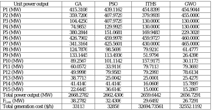
The best fuel cost result obtained from proposed GWO and other optimization algorithms are compared in Table 5 for load demands of 2630 MW. In Table 5, generation outputs and corresponding fuel cost and losses obtained by the proposed GWO are compared with those of GA, PSO, and ITHS [18, 19]. The proposed GWO provide better solution (total generation cost of 32552.1192 $/h and power losses of 26.7291 MW) than other methods while satisfying the system constraints. We have also observed that the solutions by GWO always are satisfied with the equality and
Iteration
0 20 40 60 80 100 120 140 160 180 200 104
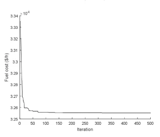
inequality constraints by using the proposed constraint-handling approach. A convergence characteristic of fifteen-generator system is shown in Fig. 2.
Table 4Fuel cost cooefficients and power limits(15-units)
Unit Pi, min (MW) Pi, max (MW) a b c e f
1 150 455 0.000299 10.1 671 100 0.084
2 150 455 0.000183 10.2 574 100 0.084
3 20 130 0.001126 8.8 374 100 0.084
4 20 130 0.001126 8.8 374 150 0.063
5 150 470 0.000205 10.4 461 120 0.077
6 135 460 0.000301 10.1 630 100 0.084
7 135 465 0.000364 9.8 548 200 0.042
8 60 300 0.000338 11.2 227 200 0.042
9 25 162 0.000807 11.2 173 200 0.042
10 25 160 0.001203 10.7 175 200 0.042
11 20 80 0.003586 10.2 186 200 0.042
12 20 80 0.005513 9.9 230 200 0.042
13 25 85 0.000371 13.1 225 300 0.035
14 15 55 0.001929 12.1 309 300 0.035
15 15 55 0.004447 12.4 323 300 0.035
Table 5 Best solution of 15-unit systems (PD = 2630 MW)
Unit power output GA PSO ITHS GWO
P1 (MW) 415.3108 439.1162 454.8399 454.9044
P2 (MW) 359.7206 407.9729 379.9939 455.0000
P3 (MW) 104.4250 407.9729 130.0000 130.0000
P4 (MW) 74.9853 129.9925 130.0000 130.0000
P5 (MW) 380.2844 151.0681 169.9483 229.3028
P6 (MW) 426.7902 459.9978 459.9727 460.0000
P7 (MW) 341.3164 425.5601 430.0000 465.0000
P8 (MW) 124.7876 98.5699 79.9210 61.4777
P9 (MW) 133.1445 113.4936 51.9794 26.4398
P10 (MW) 89.2567 101.1142 157.9175 30.1173
P11 (MW) 60.0572 33.9116 79.7113 79.3693
P12 (MW) 49.9998 79.9583 79.2993 78.6134
P13 (MW) 38.7713 25.0042 25.0001 25.4279
P14 (MW) 41.4140 41.4140 16.0608 15.7897
P15 (MW) 22.6445 36.6140 15.0000 15.2867
Total power output (MW) 2668.2782 2662.4306 2659.6442 2656.7291
PLoss (MW) 38.2782 32.4306 29.6492 26.7291
Fig. 2 Convergence characteristic by GWO for fifteen-generator system
V.CONCLUSION
This paper presents a new approach for solving ELD problems with valve-point effects using GWO technique. The GWO technique has provided the global solution in the 6-unit, and 15-unit test system and the better solution than the previous studies reported in literature. Also, the equality and inequality constraints treatment methods have always provided the solutions satisfying the constraints. Although the proposed GWO algorithm had been successfully applied to ELD with valve-point effects, the practical ELD problems should consider multiple fuels as well as prohibited operating zones. This remains a challenge for future work.
REFERENCES
[1] A. J. Wood and B. F. Wollenberg, Power Generation, Operation, and Control,New York:2nd ed., John Wiley and Sons, 1996.
[2] Z. X. Liang and J. D. Glover, “A zoom feature for a dynamic programming solution to economic dispatch including transmission losses”, IEEE Transactions on Power Systems, vol. 7, no. 2, pp. 544-550, 1992.
[3] P. H. Chen and H. C. Chang, “Large-scale economic dispatch by genetic algorithm”, IEEE Transactions on Power Systems, vol. 10, no. 4, pp. 1919-1926, 1995.
[4] C. L. Chiang, “Improved genetic algorithm for power economic dispatch of units with valve-point effects and multiple fuels”, IEEE Transactions on Power Systems, vol. 20, no. 4, pp. 1690-1699, 2005.
[5] W. M. Lin, F. S. Cheng and M. T. Tsay, “An improved tabu search for economic dispatch with multiple minima”, IEEE Transactions on Power Systems, vol. 17, no. 1, pp. 108-112, 2002.
[6] K. P. Wong and C. C. Fung, “Simulated annealing based economic dispatch algorithm”, Proc. Inst.Elect. Eng. C, vol. 140, no. 6, pp. 509-515, 1993.
[7] J. H. Park, Y. S. Kim, I. K. Eom and K. Y. Lee, “Economic load dispatch for piecewise quadratic cost function using Hopfield neural network”, IEEE Transactions on Power Systems, vol. 8, no. 3, pp. 1030-1038, 1993.
[8] K. Y. Lee, A. Sode-Yome and J. H. Park, Adaptive Hopfield neural network for economic load dispatch, IEEE Transactions on Power Systems, vol. 13, no. 2, pp. 519-526, 1998.
[9] T. Jayabarathi and G. Sadasivam, “Evolutionary programming-based economic dispatch for units with multiple fuel options”, European Trans. Elect.Power, vol. 10, no. 3, pp. 167-170, 2000.
[11] H. T. Yang, P. C. Yang and C. L. Huang, “Evolutionary programming based economic dispatch for units with non-smooth fuel cost functions”, IEEE Transactions on Power Systems, vol. 11, no. 1, pp. 112-118, 1996.
[12] Z. L. Gaing, “Particle swarm optimization to solving the economic dispatch considering the generator constraints”, IEEE Transactions on Power Systems, vol. 18, no. 3, pp. 1187-1195, 2003.
[13] J. B. Park, K. S. Lee, J. R. Shin and K. Y. Lee, “A particle swarm optimization for economic dispatch with nonsmooth cost functions”, IEEE Transactions on Power Systems, vol. 20, no. 1, pp. 34-42, 2005.
[14] J. B. Park, Y. W. Jeong, J. R. Shin, K. Y. Lee and J. H. Kim, “A hybrid particle swarm optimization employing crossover operation for economic dispatch problems with valve-point effects”, Engineering Intelligent Systems forElectrical Engineering and Communications, vol. 15, no. 2, pp. 29-34, 2007.
[15] Shi Yao Lim, Mohammad Montakhab and Hassan Nouri, “Economic dispatch of power system using particle swarm optimization with constriction factor”, International Journal of Innovations in Energy Systems and Power, vol. 4, no. 2, pp. 29-34, 2009.
[16] L. S. Coelho and C.S. Lee,“Solving economic load dispatch problems in power systems using chaotic and Gaussian particle swarm optimization approaches”, Electric Power and Energy Systems, vol.30, pp. 297–307, 2008.
[17] A. I. Selvakumar and K. Tanushkodi, “A new particle swarm optimization solution to nonconvex economic dispatch problems”, IEEE Transactions on Power Systems, vol. 22, no. 1, pp. 42–51, Feb. 2007.
[18] G. Shabib, A.G. Mesalam and A.M. Rashwan,“Modified particle swarm optimization for economic load dispatch with valve-point effects and transmission losses”, Current Development in Artificial Intelligence, vol. 2, no. 1, pp. 39-49, 2011.
[19] A. Hatefi and R. Kazemzadeh, “Intelligent Tuned Harmony Search for Solving EconomicDispatch Problem with Valve-point Effects and Prohibited Operating Zones”, Journal of Operation and Automation in Power Engineering, vol. 1, no. 2, pp. 84-95, 2013.