Image Denoising Techniques Using Dual Tree
Complex and Hyperanalytic Wavelet
Transform With Bi-Shrink Filter
S. Swarnalatha1, Dr. P. Satyanarayana2, B. Shoban Babu3
Associate Professor, Dept of E.C.E., S.V.U.C.E., Tirupati. A.P, India1 Professor, Dept of E.C.E., A.I.T.S, Tirupati, A.P, India2 Associate Professor, Dept. of E.C.E., S.V.C.E.T., Chittoor, A.P, India3
ABSTRACT: This paper focuses on the comparison of the image denoising techniques using two different complex wavelet transforms namely Dual Tree Complex Wavelet Transform (DTCWT) and Hyperanalytic Wavelet Transform (HWT). The limitations of Discrete Wavelet Transform (DWT) such as, poor shift sensitivity and poor directionality are overcome by using the complex wavelet transforms, thus, complex wavelet transforms are preferred to DWTs in the signal or image processing techniques. This paper presents the quantitative comparison of the performances of DTCWT and HWT based image denoising techniques, by using the bivariate shrinkage technique for filtering the noisy wavelet coefficients.
KEYWORDS: Discrete Wavelet Transform (DWT), Dual Tree Complex Wavelet Transform (DTCWT), Hyperanalytic Wavelet Transform (HWT), Bi-shrink Filter.
I.INTRODUCTION
During acquisition and transmission, images are often corrupted by additive noise that can be modelled as Gaussian most of the time. As an important pre-processing method, image denoising has great influence on the subsequent image analysis, for example, the accuracy of image segmentation will be influenced by the results of image denoising. The aim of image denoising algorithm is to reduce the noise level, while preserving the image features. David Donoho introduced the word denoising in association with the wavelet theory [1]. The image denoising is achieved in three steps:
i. Computation of forward Wavelet Transform, ii. Filtering the wavelet coefficients, and
iii. Computing inverse Wavelet transform with filtered wavelet coefficients.
As the Discrete Wavelet Transform suffers from the poor shift sensitivity and poor directional selectivity [2], there is a strong need for new wavelets which overcomes the limitation of DWT. In this paper, two different complex wavelet transform techniques, namely, Dual Tree Complex Wavelet Transform (DTCWT) and Hyperanalytic Wavelet Transform (HWT) are presented, which have high degree of sensitivity and improved directionality. These features of complex wavelet transforms are utilized in the image denoising.
II.DUAL TREE COMPLEX WAVELET TRANSFORM (DTCWT)
Fig 1. Analysis Filter Bank of DTCWT
For the filter bank structure, shown in Fig 1, let h0 and h1 represent CQF (Conjugate Quadrature Filter) pair [4 – 6]. That
is,
ℎ
( ) = (
−
1)
ℎ
(1
−
)
. . . (1)
and in Z-transform domain
( )
(
) +
( )
(
) = 2
. . . (2)
( ) =
(
)
. . . (3)
The real tree and imaginary tree scaling and wavelet functions form the Hilbert Transform pairs. If ( ), ψ ( ), ( ) and ψ ( )are the scaling and wavelet functions of real and imaginary trees, the relation between the real and imaginary scaling and wavelet functions is given by
( ) =
{
( )}
ψ
( ) =
{
ψ
( )}
. . . (4)
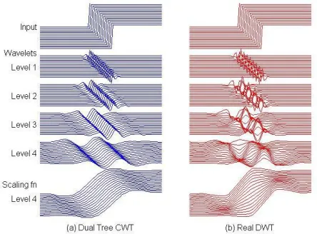
DTCWT has approximate shift-invariance, or in other words, improved time-shift sensitivity in comparison with standard DWT. The reconstructed details at various levels and approximation at the last level have almost uniform shifts for the time-shifted unit step functions [6]. The shift sensitive nature of DTCWT is illustrated in the Fig. 2 and from this figure, it is obvious that the shift sensitivity of real DWT is poorer than that of DTCWT.
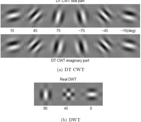
Standard DWT offers the feature selectivity in only three directions with poor selectivity for diagonal features, whereas DTCWT has twelve directional details (6 for each of real and imaginary trees) oriented at angles ±15, ±45, ±75 of in 2-D as shown in Fig 3. From this figure, is clear that, the 2-DWT provides three directions of information in the details, whereas the DTCWT provides twelve directions of information in the details.
Fig 3. Interpretation of Directional Selectivity of DTCWT
III. HYPERANALYTIC WAVELET TRANSFORM (HWT)
In Dual Tree Complex Wavelet Transform, one is required to design the low pass, high pass FIR filters for both real tree and imaginary tree, such that the scaling and wavelet functions of real and imaginary trees form a Hilbert Transform pair. It means, that the filters of DTCWT are designed with some more constraints than in the filters of classical wavelet transforms. Instead of designing the complex filters which is not easy task, it is better to process the complex signal or image (Analyticity) corresponding to the given signal or image, using classical wavelets.
Given a real signal ( )we can construct the complex (analytic) signal as ( ) = ( ) + { ( )} . . . (5)
The new implementation of complex wavelet transform of the signal ( ) is given as
Fig. 4. Implementation of Analytic (Complex) Wavelet Transform (AWT)
From this implementation of AWT [7], the wavelet coefficients of ADWT as follow, =〈 ( ), ( )〉
=〈 ( ) + { ( )}, ( )〉. . . (6)
Where ( )is the analytic (complex) signal corresponding ( ), ( )is the classical wavelet.
For one dimensional signal, the analytic signal can be computed with the help of Hilbert Transform along the length of the signal. But, for 2D-signal like image, its analytic signal is computed by finding the Hilbert Transform along the rows, columns and both rows and columns of the image.
DWT ( )
The two dimensional implementation of Analytic Wavelet Transform is called Hyperanalytic Wavelet Transform (HWT). The Hyperanalytic Wavelet Transform (HWT) [7 – 9] of an image ( , ) is
{ ( , )} =〈 ( , ), ( , )〉+ 〈 ( , ), { ( , )}〉+ 〈 ( , ), { ( , )}〉
+ 〈 ( , ), { ( , )} 〉
Where = = = =− , =− = , =− = , =− =
⇒ { ( , )} =〈 ( , ), ( , )〉+ 〈 { ( , )}, ( , )〉+ 〈 { ( , )}, ( , )〉+
〈 { ( , )} , ( , )〉
⇒ { ( , )} = { ( , )} + { ( , )} + { ( , )} +
{ ( , )}
Here 〈 ( , ), ( , )〉= { ( , )}. . . (7)
Fig. 5. Implementation of HWT
From the equation (7), it is obvious that, Hyperanalytic Wavelet Transform (HWT) of the image ( , ) can be computed with the aid of two dimensional Discrete Wavelet Transforms (2D-DWT) of its associated hypercomplex image. In consequence the HWT implementation uses four trees, each one implementing a 2D-DWT, thus having a redundancy of four. The first tree is applied to the input image. The second and the third trees are applied to 1D-Hilbert transforms computed across the lines ( )or columns ( )of the input image. The fourth tree is applied to the result obtained after the computation of the two 1D Hilbert transforms of the input image. The HWT implementation [7 – 8] is presented in Fig. 5.
Fig. 6. Comparison of shift invariance nature of AWT, DTCWT, real DWT
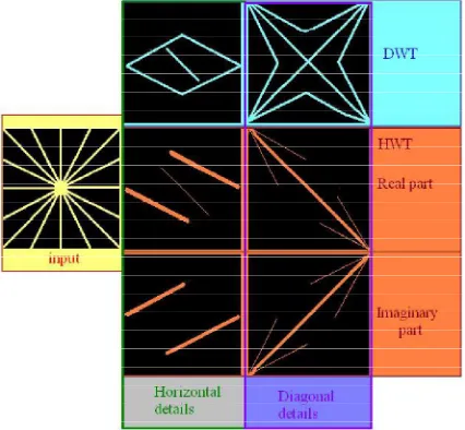
Like the 2D DTCWT, the HWT implemented as proposed in Fig 5, has six preferential orientations: ± Tan-1(1/2), ±π/4 and ± Tan-1(2). The 2D-DWT has only three preferential orientations: 0, ±π/4 and π/2, it does not make the difference between the two principal diagonals [7 – 9]. The better directional selectivity of the proposed implementation of HWT versus the 2D DWT can be easily observed, comparing the corresponding detail sub-images in Fig 7.
Fig. 7. Illustration of Directionality of HWT
IV.IMAGE DENOISING
In common use, the word ‘noise’ refers to any unwanted sound. In both analog and digital electronics, noise is an unwanted perturbation to a wanted signal; it is called noise as a generalization of the audible noise heard when listening to a weak radio transmission. Signal noise is heard as acoustic noise if played through a loudspeaker and it manifests as ’snow’ on a television or video image. Noise can block, distort, change or interfere with the meaning of a message in both human and electronic communication. In signal processing or computing it can be considered unwanted data without meaning; that is, data that is not being used to transmit a signal, but is simply produced as an unwanted by-product of other activities.
Johnstone. The new shrinkage function, which depends on both the coefficient and its parent, yields improved results for wavelet-based image denoising
.
Let represent the parent of ( is the wavelet coefficient at the same spatial position as , but at the next coarser scale).Then = +
where = + , = + = + . The noise values , are zero-mean Gaussian with variance sigma2. Based on the empirical histograms that we have computed, we propose the following non-Gaussian bivariate [9 – 10] Probability Density Function (pdf)
( ) = 3
2 exp −
√3 +
With this pdf, and are uncorrelated, but not independent. The MAP estimator of yields the following bivariate shrinkage function [9 – 10]
=( + −
√ )
+ . 1
For this bivariate shrinkage function, the smaller the parent value, the greater the shrinkage. The algorithm of this work is
(a) Consider an original Image (noise free)
(b) Generate the noisy images (Gaussian) with different values of standard deviation (c) For each noisy image, apply DTCWT and HWT techniques.
(d) Filter the detail coefficients of the both DTCWT and HWT, using bivariate shrinkage technique. (e) Apply the inverse DTCWT and HWT for the filtered coefficients to get denoised images.
(f) Compute the Mean Square Error (MSE) and Peak Signal to Noise Ratio (PSNR) of the denoised images with respect to the original image
(g) Tabulate the MSE and PSNR for different amount of noises, for different wavelet techniques.
The Mean Square Error (MSE) is calculated by using the following equation,
where, ( , )is the input, noise free image, ( , )is the output image, may be noisy or denoised, and M, N are the number of rows and columns of the image, respectively.
The Peak Signal to Noise Ratio (PSNR) is being computed using the following equation,
where, R is the maximum fluctuation in the input image data type. For example, if the input image has a double-precision floating-point data type, then R is 1. If it has an 8-bit unsigned integer data type, R is 255.
V. RESULT AND DISCUSSION
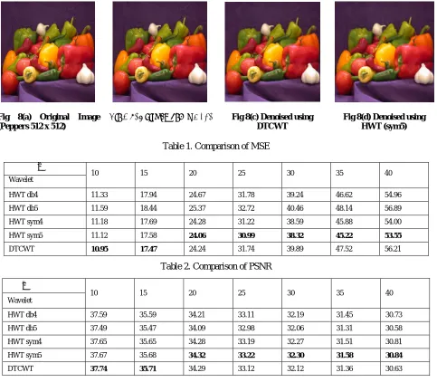
The performance of the DTCWT and HWT based denoising techniques analysed for the ‘Peppers’ image of 512 x 512 dimensions. The image is added with Gaussian noise with the variances ranging from σ = 10 to 40 in steps of 5. Noise free ‘Peppers’ image is shown in the Fig 8 (a) and noisy ‘Peppers’ image with σ = 30 is shown in the Fig 8 (b).
The HWT technique is implemented using four different wavelets, viz. ‘db4’, ‘db5’, ‘sym4’, and ‘sym5’.The noisy ‘Peppers’ image is subjected six levels of DTCWT and HWT decomposition techniques, so that the approximation wavelets coefficients are not severely affected with the noise.
The details coefficients of the each stage are filtered using bivariate shrinkage technique. Thus, filtered wavelets are subjected to the corresponding inverse DTCWT and inverse HWT techniques in order to obtain the denoised images. The performance metrics MSE and PSNR are tabulated in the Tables 1 and 2 respectively. For graphical interpretation,
=∑ | ( , )− ( , )| ,
,
.
MSE and PSNR values are represented as bar graphs for the different values of σ. The denoised images using DTCWT and HWT with ‘sym5’ are shown in the Fig 8 (c) and Fig. 8 (d) respectively.
Fig 8(a) Original Image (Peppers 512 x 512)
Fig 8(b) Noisy Image (σ = 30) Fig 8(c) Denoised using
DTCWT
Fig 8(d) Denoised using HWT (sym5)
Table 1. Comparison of MSE
σ
10 15 20 25 30 35 40
Wavelet
HWT db4 11.33 17.94 24.67 31.78 39.24 46.62 54.96
HWT db5 11.59 18.44 25.37 32.72 40.46 48.14 56.89
HWT sym4 11.18 17.69 24.28 31.22 38.59 45.88 54.00
HWT sym5 11.12 17.58 24.06 30.99 38.32 45.22 53.55
DTCWT 10.95 17.47 24.24 31.74 39.89 47.52 56.21
Table 2. Comparison of PSNR
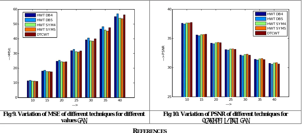
From the Tables 1 and 2, and Figures 9 and 10, the following can be observed:
(a)In the HWT based denoising technique, the wavelet ‘sym5’ outperforms than the remaining wavelets, viz., ‘db4’, ‘db5’ and ‘sym4’, for all the values of standard deviation of Gaussian noise added. (b)For low values of standard deviation of Gaussian noise added (σ < 20), the DTCWT based denoising
techniquesperforms better than the HWT of any wavelet.
(c)At high values of standard deviation of Gaussian noise added (σ > 20), HWT with ‘sym5’ performs better than the DTCWT.
σ
10 15 20 25 30 35 40
Wavelet
HWT db4 37.59 35.59 34.21 33.11 32.19 31.45 30.73
HWT db5 37.49 35.47 34.09 32.98 32.06 31.31 30.58
HWT sym4 37.65 35.65 34.28 33.19 32.27 31.51 30.81
HWT sym5 37.67 35.68 34.32 33.22 32.30 31.58 30.84
In summary, one can easily observe that DTCWT based technique is denoising effectively the images corrupted with less noise. Though DTCWT based denoising performs better than the DWT based denoising technique at all levels of noise but at high amounts of noise, HWT based techniques better than the DTCWT based techniques.
VI.CONCLUSION
This paper compares the denoising capability of the DTCWT and HWT based techniques implemented bivariate shrinkage method. From the results and performance metrics, it can be concluded that DTCWT based denoising techniques are preferred at low levels of noise and HWT based denoising techniques are preferred at high levels of noise. Though this paper is limited to Gaussian noise, this generalization can be extended to any type of noise, because sum of the independent noises tends to Gaussian distribution.
REFERENCES
[1] D. L. Donoho, I. M. Johnstone, Ideal spatial adaptation by wavelet shrinkage, Biometrika, 81(3): pp. 425-455, 1994.
[2] N. Kingsbury, Complex Wavelets for Shift Invariant Analysis and Filtering of Signals, Applied and Comp. Harm. Anal.10, 2001, pp. 234-253. [3] N G Kingsbury, A Dual-Tree Complex Wavelet Transform with improved orthogonality and symmetry properties, Proc. IEEE Conf. on Image Processing, Vancouver, September 11-13, 2000, paper 1429.
[4] Ivan W. Selesnick. The Characterization and Design of Hilbert Transform Pairs of Wavelet Bases. In 2001 Conference on Information Science and Systems, The Johns Hopkins University, 2001
[5] N. Kingsbury, “Image processing with complex wavelets”, Philosophical Transactions of the Royal Society London A 357 no.1760 :2543-2560, 1999.
[6] Ivan W. Selesnick, Richard G. Baraniuk and Nick G. Kingsbury. The Dual-Tree Complex Wavelet Transform. IEEE Signal Processing Magazine, 22(6) : pp. 123-151,2005.
[7] C. Nafornita, I. Firoiu, J. Boucher, A. Isar “A New Watermarking Method Based on the use of the Hyperanalytic Wavelet Transform” [8] I. Firoiu, C. Nafornita, “Image Denoising using a New Implementation of Hyperanalytic Wavelet Transform”, IEEE Trans. on Instrum. And Meas., Vol. 58, no. 8, pp. 2410-2416, 2009.
[9] I. Adam, C. Nafornita, J-M Boucher and A. Isar, “A Bayesian Approach of Hyperanalytic Wavelet Transform Based Denoising”. [10] L. Sendur and I. W. Selesnick, “Bivariate shrinkage functions for wavelet-based denoising exploiting interscale dependency”, IEEE Trans. on Sign. Proc. Vol. 50 no. 11, pp. 2744-2756, 2002.
[11] I. Firoiu, A. Isar, and D. Isar, “A maximum A Posteriori Approach of Hyperanalytic Wavelet Based Image Denoising in a Multi-Wavelet Contenet’.
[12] Massimo Fierro, Ho-Gun Ha, and Yeong-Ho Ha “Noise Reduction Based on Partial-Reference, Dual-Tree Complex Wavelet Transform Shrinkage”, IEEE Trans. on Image Proc. vol. 22, no. 5, may 2013 pp. 1859-1872.
Fig 9. Variation of MSE of different techniques for different values of σ
Fig 10. Variation of PSNR of different techniques for
different values of σ
10 15 20 25 30 35 40
0 10 20 30 40 50 60 ---> ---> M S E HWT DB4 HWT DB5 HWT SYM4 HWT SYM5 DTCWT
10 15 20 25 30 35 40
25 30 35 40
--->
BIOGRAPHY
Mrs. S. Swarnalatha received her graduation degree in Electronics and Communication Engineering from JNTUCEA (JNTU) in 2000, received post-graduation degree in digital electronics and communication systems from JNTUCEA (JNTU) in 2004 and pursuing Ph.D. from SVUCE (SVU) Tirupati in the image processing domain. I worked as lecturer at JNTUCEA, Anantapur for 4 years, worked as Assistant and Associate professor in the department of ECE, at MITS, Madanapalle, worked as Associate professor at CMRIT, Hyderabad and presently working as Associate Professor at SVUCE (SVU), Tirupati.
Email:[email protected]
Prof. P. SATYANARAYANA received his Bachelor’s Degree in Electronics and Communication Engineering from SVUCE (SVU) in 1976, he received his Master’s Degree in Instrumentation and Control System from SVUCE (SVU) in 1978 and he received his Doctorate in Digital signal Processing 1987 from SVUCE (SVU) in 1987. He is the Post-Doctoral Fellow in Department of Electrical & Computer Engineering at Concordia University, Montreal, Canada during 1988 to 1990. He worked as Visiting Faculty in the School of Aerospace Engineering, University Science Malaysia, Pinang, Malaysia from 2004 to 2007. He visited number counties like USA, Canada, Malaysia, Singapore, and England to have academic and cultural exchange. He started his career as lecturer from 1976 with the home University SVUCE (SVU), as Associate professor during 1991-1999, as professor during 1999-2013 in department of Electronics and Communication Engineering, Tirupati. He is presently working as professor in ECE at AITS, Tirupati.