Influence
of Natural Mulch on Forage Pro-
duction on Differing California Annual Range
Sites
JAMES VI/. BARTOLOME, MICHAEL C. STROUD, AND HAROLD F. HEADY
Abstract
Manipulation of natural mulch on nine experimental plots in California annual grassland representing a range of mean annual precipitation from I60 to 16 cm provided information useful for grazing management. Peak standing crop correlated highly significantly with precipitation. Response of peak standing crop to five levels of natural mulch ranging from zero to 1,120 kg/ha differed with site. Three types of sites distinguished by mean annual precipitation and plant species composition were identi- fied. On sites with significant numbers of perennial grasses and more than 150 cm of mean annual precipitation, maximum standing crop is reached when more than 1,120 kg/ha of mulch is present on the ground at the beginning of the fall growing season. Peak standing crop results from 840 kg/ha of mulch on sites containing the annuals Bromus mollis and Erodium botrys and with between 100 and 65 cm of mean annual precipitation. Mulch did not significantly influence standing crop in regions dominated by Bromus rubens and Erodium cicutarium and receiving less than 25 cm of mean annual precipitation. Annual grassland response to mulch and grazing is highly site specific, yet the resilience of annual rangelands also allows rapid recovery from overuse.
A distinctive combination of use by people and the influence of geography and climate fostered the formation of the present California annual grassland. The vegetation is dominated primarily by annual grasses of Mediterranean origin, which replaced the native bunchgrasses during the 19th century. Reflecting the diverse geography of the state, the California annual grassland varies in productivity, component species, and the degree of replacement of the native plants by aliens. The climate, although generally typically Mediterrean with cool wet winters and dry summers, varies for example, in average annual rainfall, from nearly 200 cm (80 inches) in the North Coast to less than 15 cm (6 inches) in the rainshadow of the South Coast ranges.
The growth of vegetation follows a characteristic pattern. In response to fall rains, plants establish from seed produced the previous spring. Slow vegetative growth and root development in the cool winter months are followed by rapid growth with warming temperatures in spring. Maximum annual standing crop generally occurs in late spring. In summer only the seeds are left as living agents to repeat this process again in the fall.
The authors are lecturer and associate specialist, Department of Forestry and Resource Management, University of California, Berkeley, 94720; conservationist (civilian), Department of the Navy, Western Div., Naval Facilities Engineering Command, San Bruno, California 94066; and assistant vice president, Division of Agricultural Sciences, University of California, Berkeley 94720.
Glen D. Savelle established and experimental plots and carried out the initial treatments and sampling. Michael D. Pitt contributed significantly to later sampling and plot manipulation. The cooperation of private and public landholders is gratefully acknowledged.
Manuscript received November 20, 1978.
4
Much of California’s range livestock industry relies on the yearly rejuvenating capability of the annual range. Indeed, most of California’s big game and upland wildlife populations rely on the annual forage crop for significant portions of their diet. The titure of these valuable resources and capital investments need not be wholly entrusted to the whims of nature’s erratically patterned and oftentimes meager rainfall. The purpose of this study was to show how prudent and knowledgeable seasonal management of the mulch layer in conjunction with an understanding of site differences over California’s 6 million hectares of annual range can significantly influence the subsequent year’s forage production.
The 6 million hectares of grassland in California (Barbour and Major 1977) extend nearly the entire length of the state. Stand composition and productivity vary considerably over the grassland. Munz and Keck ( 1949) divided the grassland into two plant communities, the Coastal Prairie and the Valley Grassland. Kiichler’s (1964) Fescue-Oatgrass and California Steppe vegetation types as updated into Coastal Prairie-Scrub Mosaic and Valley grassland (Ktichler 1977) retain the basic divisions of Munz and Keck.
Detailed descriptions of species composition within the annual grassland remain scarce. Burcham (1975) reported abundance of annual grassland species from 38 plots in the Sierra foothills from Sacramento to Madera County and in the Coast ranges from Santa Clara to Monterey County. Species of
Bromus and Erodium exhibited a high degree of constancy. Soft chess (Bromus mollis) formed a significant amount of the vegetative cover on 30 plots and was absent on only one plot. Ripgut brome (Bromus rigidus), although a significant percentage of the cover on only one plot, occurred on 2 1 plots.
Erodium species were present on 3 1 plots, forming a significant portion of the cover on 28 plots.
Janes (1969) sampled species composition on the western side of the Central Valley and in the North Coast ranges along an average annual precipitation gradient ranging from 12.5 to 200 cm and also showed soft chess to be the most widely distributed annual grassland species. Janes encountered 124 species at his 20 sample locations, yet only seven species occurred at more than four locations. Soft chess occurred at 15 sites, ripgut brome at 11 sites, and broad-leaved filaree (Erodium botrys) at 7 sites. Janes’ study in the spring of 1969 remains the only comprehensive survey of geographical variation in the annual grassland.
Understanding site variation in annual grassland is necessary for effective management. Composition and productivity of annual ranges vary remarkably between and within years.
Talbot et al. ( 1939) and Bentley and Talbot ( 195 1) provided several years of data on yearly variations in composition and production of annual grassland at the U.S. Forest Service- operated San Joaquin Experimental Range (50 km north of Fresno), a site with continuous documentation since the early
1930’s (Duncan and Woodmansee 1975). Composition and productivity at the University of California’s Hopland Field Station has been monitored since the early 1950’s with documentation of variations within the year (Heady 1958; Bartolome 1978; Savelle 1977) and yearly long-term production and composition (Murphy 1970; Pitt and Heady 1978) in relation to weather patterns. Consideration of sites apart from the San Joaquin Range and Hopland are few, including Evans et al. ( 1975) at the University of California’s Sierra Foothill Range
100 km north of Sacramento, Batzli and Pitelka (1970), and Raliff and Heady (1962) near San Francisco Bay in Alameda County.
The impacts of grazing by livestock on annual grassland have not often been directly investigated. Elliot and Wehausen (1974) examined response of coastal prairie species to grazing on Point Reyes. A long-term grazing study at the San Joaquin Experimental Range enabled the development of management guidelines for annual range (Bentley and Talbot 195 1). Hedrick (1948) also looked at the effects of grazing intensity on annual range. Most of the response of annual gr_assland species to grazing has been inferred from experiments simulating grazing through the removal of varying amounts of plant residue or mulch (Talbot et al. 1939; Heady 1956). Experiments at Hopland showed a response of the grassland to mulch manipulation similar to that which would be expected under livestock grazing (Heady 196 1). These results were extended to a discussion of economic factors (Hooper and Heady 1970) involved in intensity of mulch removal on annual grassland. Mechanisms explaining the effects of mulch have not been demonstrated, but several factors probably are important. Soil organic matter and bulk density are both improved with increasing amounts of mulch, but only in the upper few inches of the soil (Heady 1966). Mulch protects the soil surface from erosion and provides a favorable environment for plant growth.
70
o Fresno \’
200km IFig. 1. Mup oj Culijorniu showing location oj nine study plots
Several authors have ascribed the differences in botanical composition due to manipulation of mulch to the effect on plant establishment (Bartolome 1978; Evans and Young 1970; Tinnin and Muller 197 1).
Methods
Figure 1 shows the locations of the nine plots in relation to major cities in California. A summary of specific site information on location, geography, rainfall, and soils is provided in Table I. The plot sites were chosen to represent differing climatic types that support significant portions of the California annual range type.
The experimental treatments consisted of removal of mulch or plant residue to a fixed, predetermined level. Mulch manipulations were applied in late summer or early fall prior to the onset of the rainy season. Since the first rains of the season stimulating fall germination
Table 1. Location, geography, rainfall, and soils information for the study plots.
Cm of Average
annual rainfall Soil
Plot Plot name Type of Long Study Elevation Soil depth
number (county) ownership term period (M) Latitude texture (M)
1 May Rant h Private 150 155 640 40” 25’N Clay loam l-l.2
(Humboldt)
2 Bear River Ridge Private 150 177 670 40” 30’N Clay loam l-l.2
(Humboldt)
3 Albee Ranch Private 160 144 550 40” 20’N Loam 0.6-l
(Humboldt)
4 Hopland Field Station University of 100 96 305 39” OO’N Fine sandy 0.6-l
(Mendocino) California loam
5 Jeffers Ranch Private 65 62 365 39” 55’N Light clay 0.3-0.6
(Tehama) IOZUIl
6 Russell Reservation University of 65 65 215 37” 50’N Clay 1.5-1.8
(Contra Costa) California
7 Panache Hills Bureau of Land 20 24 455 36” 40’N Sandy loam 0.3-0.6
(Fresno) Management
8 Kettleman Hills Bureau of Land 16 17 215 36” 05’N Fine sandy 0.6-l
(Fresno) Management
9 Temblor Range Bureau of Land 20 21 760 35” OO’N Sandy loam 0.3-0.6
below comprise important plant groups both from the standpoint of forage production and as indicators of the overall variation in botanical composition throughout the annual grassland.
Site Classification
Location of the nine study plots reflected estimated average annual precipitation along a mean annual precipitation gradient from 160 to 16 cm. Therefore average rainfall forms the first measure of site variation between plots and constitutes the major variable explaining variation in peak standing crop and total vegetative cover as determined by regression analysis (Table 2). The linear conelation between average annual precipitation and standing crop (I = 0.7572) is somewhat better below 100 cm mean annual precipitation (Fig. 3). Although rainfall increased 60% between Hopland (Site 4) and Albee Ranch (Site 3) for example, standing crop increased only about 20%. This result suggests that effective rainfall, resulting in increased plant growth, drops off above approximately 100 cm. Cover shows a response similar to that of standing crop
usually come earlier at the northern most plots, these were manipulated first. Mulch treatments were applied to the other plots in essentially their numbered order. Mulch manipulation treatments were intended to be applied to each plot for five successive years. Treatments were initiated on plots I, 2,4, and 5 in the fall of 1967, on plots 3 and 6 in the fall of 1968, and on plots 7.8, and 9 in the fall of 1969. Treatments continued for only 3 years on plots 7, 8, and 9. Treatment squares were 3 by 3 meten (10 x 10 ft) and arranged in a 5 X 5 latin square (five replications of five treatments). The square was mowed to a uniform stubble height of about 10 cm, then clipped by hand to establish the desired quantity of mulch. Treatment levels measured “zero ” 280, 560, 840, and 1,120 oven-dry kg per hectare (0, 250, 500, 7;0, loo0 lb/ acre o mu c remaining (Fig. 2). Each ) f I h square received the same treatment each year throughout the study period. After handclipping to approximately the desired level, two 30
X 30 cm (l-foot square) samples were clipped to ground level and weighed. Addition or subtraction of mulch resulted in the desired residue plus or minus an allowable error of 10%. Care was taken to avoid disturbing the soil surface, thus the treatment of “zero” pounds per acre represents a slightly greater amount. The “zero” mulch treatments constituted the base or standard for the other treatments. That is, the 280 kg treatment was applied on top of the small, comparable amount that remained in the “zero” plots. After all adjustments had been made, a 30 x 30 cm (sq. ft.) sample was taken and returned to the laboratory to determine the actual moisture-free amount of mulch applied. This amount was usually within a range of 25 kg per hectare on either side of the prescribed treatment.
Once a year at or near the time of maximum biomass (mid-April in the south to mid-June in the north), samples were clipped and oven dried to determine standing crop, the most convenient estimate of plant productivity. Recorded locations of all clipped samples prevented resampling the same square foot in subsequent years. The treatment squares were sampled for species composition and plant foliar cover, using the New Zealand-developed ten-point frame (Heady and Rader 1958). Species composition, indicated by the first hit, was measured in the middle of the treatment square where herbage samples were never taken. Species chosen for detailed discussion
Species composition reflects the components of productivity on a site. Forage composition may be considered a further retinement of site characteristics as manifested in the vegetation. Although the flora of an individual study plot often included 50 or more species, five species groups will be discussed in this section. Figure 4 gives an example of variation in species composition at different locations. The most striking discontinuity in species distribution involves the replacement of soft chess and broad-leaved tilaree with red brome (Bromus rubens) and red-stem iilaree (Erodium cicurarium),
respectively, on the three driest sites (plots 7.9). all with 25 cm or less of annual rainfall. Plots 4 and 5, receiving 100 and 65 cm mean annual precipitation, respectively, are both characterized by broad-leaved FiLxee, soft chess, and few orno perennial grasses. Site 6contained no &u~e species and was the only site with annual barley (Hordeurn) species. fhe three wettest sites (plots 1-3) with greater than 150 cm
Independent vtiable Ftoenterorremove
Location 1271.385
Mulch trea”nent 73.228
Row 0.055
Gl”lll” 2.607
Year 16.237
Significance
p<.M), p<.oO, p<.814 &I<.107 p<.OO1
Multiple R
0.75722 0.77856 0.77858 0.77933 0.78398
R’ change
30 I PERENNIAL GRASSES
II
ERODIUM BOTRYSg E. CICUTARIUM
56 78 9
LOCATION
Fig. 4. Percent cover contributed by selected plant groups ut nine locutions.
precipitation, all contained broadleaved filaree or soft chess. Other annual grassland species also segregate out along the broad environmental gradient represented by the nine sites. For example, the perennial California oatgrass (Dunthonia culijornicu) and the annual crested dogtail (Cynosurus echinutus) were found only on the three wettest sites.
The discussion above illustrates a further division of site based on botanical composition, which reflects historical use of a given site and may be manipulated by grazing management. Yet each site has a limited set of potential species. Rangeland dominated by red brome and red-stem filaree could be a suitable management goal on a site with less than 25 cm average annual rainfall, yet reflect past abuses and poor quality rangeland on wetter sites. Perennial grasses may be a realistic management goal in the North Coastal region (plots 1-3) but not at other locations.
Effects of Mulch Manipulation on Productivity
The determination of site potential for both forage productivi- ty and composition is necessary for evaluation of past, present, or proposed management. Within the annual grassland type little research has reported the effects of varying grazing intensities, especially on unimproved ranges. The following section describes the results of a series of mulch manipulations used to simulate the effects of varying grazing intensity on the nine study sites.
Although mulch significantly ( P c.05; Table 2) affected standing crop, this treatment explains only 3% of the overall variation in herbage productivity. The effects of mulch reflect the response of individual plants to changes in the micro- environment near the soil surface. The overall productivity and composition of the vegetation result from the summed response to individual plant species.
Within the range of treatments applied, perennial grass sites (plots l-3) responded to mulch in a manner suggesting that leaving 1,120 kg of plant residue per hectare is still too intensive a rate of defoliation (Fig. 5). Sites 2 and 3 showed large increases in productivity between 840 and 1,120 kg/ha. Thus no optimal relationship between mulch treatment and subsequent productivity can be determined. Response to treatment also reflects the perennial nature of the vegetation. Standing crop did not begin to show a consistent response to treatment until the second year of the experiment on sites l-3. The perennial grass areas need more study to determine the effects of clipping on productivity.
,
0 280 560 840
kg/ha OF MULCH
1120
Fig. 5. EfJect oj d#ering levels of nutural mulch on peak stunding crop at nine locations. Results average 5 years on plots 1-6, 3 yeurs on plots 7-9. Least signijicant dljferences between means (PC .O.S) ure 4.27 gljf for plots 1-6, 5.5 1 g/ft’ jor plots 7-9.
The middle-rainfall sites 4 and 5, dominated by annual grasses, showed peaks of productivity of 840 kg/ha of mulch remaining in the fall. Plot 6, atypically, showed the smallest percentage change in productivity due to mulch, increasing only 23% between the lowest and highest mulch treatments. The response of other annual grass plots was immediate, with the establishment of the overall pattern in the first year following initiation of the treatment. The amount of increased forage approximated the added amount of mulch required for peak production of these mesic sites.
The dry sites (plots 7, 8, 9) varied in reponse to mulch, with the Kettleman Hills site (plot 8) showing a 106% increase with 1,120 kg/ha versus zero treatment (Fig. 5). However, for all three sites production in a given year may be well below 1,120 kg/ha. In no case did the extra mulch result in an equivalent increase in forage production.
Discussion
different seasonal production of herbage. This aspect of grassland production should be coupled with more precise measures of site variation.
Results from the manipulation of natural mulch on the study plots reflect both the characteristics of different sites and the definition of those sites. The three major site divisions each responded differently to mulch manipulation. The three most northerly perennial grassland sites illustrate the limitations of the methods used. Most perennial sites will require a seasonal defoliation study to clarify the proper intensity of grazing. Two of the three sites suggested that leaving 1,120 kg/ha (1,000 lb/acre) of mulch does not result in the optimal expression of productivity. For sites in the middle precipitation zones of 100 to 40 cm (40 to 15 inches) the optimal amount of mulch remaining is 840 kg/ha (750 lb/acre). At locations below 25 cm
(10 inches) of annual precipitation, mulch cannot be an important decision-making criterion since the response of the vegetation is highly variable.
The results of this study provide valuable insight into grazing management. Yet differences between the mulch treatments and grazing are important. The manipulation of mulch was performed in late summer or early fall, while grazing usually is heaviest in the growing season. Grazing is selective, animals also trample the soil and redistribute nutrients, while clipping does not include these factors. We believe that grazing and clipping will give the same optimal rate of grazing intensity in the middle rainfall sites in annual grassland, 840 kg/ha (750 lb/acre). On perennial sites and the low rainfall (less than 25 cm) sites, effects of grazing versus clipping diverge.
Several important conclusions, which must be site specific, may be drawn concerning grazing management on annual grassland. Differing annual range sites require different management strategies. Perennial sites with annual precipita- tion greater than 100 cm probably should be managed as perennial grassland with attention paid to plant vigor, season of grazing use, and maintenance of at least 1,120 kg/ha (1,000 lb/acre) of mulch, preferably more, at the end of the grazing season. On the mid-rainfall annual ranges, mulch is the most important factor. Proper use of these ranges would leave 840 kg/ha (750 lb/acre) of mulch at the end of the season. , Obviously, factors influencing mature plant vigor are not as important for annuals. On the drier sites, grazing management should be directed toward maintenance of sufficient plant cover to prevent soil loss; but within the constraint, animal performance can help to determine the degree of grazing intensity. Livestock often cannot graze intensively enough to reduce productivity on these dry sites without suffering performance losses as available forage drops below 560 kg/ha. Annual ranges are remarkable in their year-to-year variability in both composition and production, and therefore respond rapidly to mulch treatment. In most cases the response was apparent in the first year following treatment. This rapid response implies a great flexibility in grazing management over the majority of annual ranges. The watershed and soil protection qualities of annual ranges benefit from this resilience as well.
Although the proper mulch prescription gives the optimum production within the limitations of a given year, an immediate response means that in an extreme situation the livestock manager may use forage, foregoing some production in the next
year to obtain a benefit in the present year. An example would be a drought year where forage is short, livestock prices are low, feed prices are high. Instead of removing livestock when the optimal mulch level is reached the manager cotild instead
‘ ‘overgraze, ’ ’ knowing that in the subsequent year forage production would be reduced somewhat, but that if the next year were a high rainfall year much forage would be available, and the following year the system would return to “normal.” When the forage is needed it may be used, because the range will recovery very rapidly. Composition and production of annual ranges is dictated both by the potential of the given site, each season’s rainfall, and the appropriate management of natural mulch.
Literature Cited
Barbour, M.G., and J. Major. 1977. Introduction. In: Barbour, M.G. and J. Major (eds.) Terrestrial Vegetation of California: John Wiley and Sons, N.Y. p. 3-10.
Bartolome, J.W . 1979. Germination and establishment of plants in California annual grassland. J. Ecol. 67: (In Press)
Batzli, G.O., and F.A. Pitelka. 1970. Influence of meadow mouse popu- lations on California grassland. Ecology 51: 1027-1039.
Bentley, J.R., and M.W. Talbot. 1951. Efficient use of annual plants on cattle ranges in the California foothills. U.S. Dep. Agr. Circ. 870. 52 p. Burcham, L.T. 1975. Climate, structure, and history of California’s annual
grassland ecosystem. In: R.M. Love (ed.) The California Grassland Eco- system. Inst. Ecol., Univ. California, Davis. p. 16-34.
Duncan, D.A., and R.G. Woodmansee. 1975. Forecasting forage yield from precipitation in California’s annual rangeland. J. Range Manage. 28: 327- 329.
Elliott, H.W ., and J.D. Wehausen. 1974. Vegetational succession on coastal rangeland of Point Reyes Peninsula. Madrono 22: 231-238.
Evans, R.A., B.L. Kay, and J.A. Young. 1975. Microenvironment of a dynamic annual community in relation to range improvement. Hilgardia 43: 79-102.
Evans, R.A., and J.A. Young. 1970. Plant litter and establishment of alien annual weed species in rangeland communities. Weed Sci. 18: 697-703. Heady, H.F. 1956. Changes in a California annual plant community induced
by manipulation of natural mulch. Ecology 37: 798-812.
Heady, H.F. 1958. Vegetational changes in the California annual type. Ecology 39: 402-416.
Heady, H.F. 1961. Continuous vs. specialized grazing systems: A review and application to the California annual type. J. Range Manage. 14: 182- 193. Heady, H.F. 1966. The influence of mulch on herbage production in an
annual grassland. Proc. 9th Int. Grassl. Congr. 1: 391-394.
Heady, H.F., and L. Rader. 1958. Modifications of the point frame. J. Manage. 11: 95-96.
Hedrick, D.W. 1948. The mulch layer of California annual ranges. J. Range Manage. 1: 22-25.
Hooper, J.F., and H.F. Heady. 1970. An economic analysis of optimum rates of grazing in the California annual-type rangeland. J. Range Manage. 23: 307-3 11.
Janes, E.B. 1969. Botanical composition and productivity in the California annual grassland in relation to rainfall. M.S. Thesis. Univ. California 47 p. Kc&ler, A.W . 1964. Potential natural vegetation of the conterminous United
States. Amer. Geog. Sot. Spec. Pub. 36.
Kcchler, A.W. 1977. The map of the natural vegetation of California: In: Barbour, M.G. and J. Major (eds.) The Terestrial Vegetation of California. John Wiley and Sons, N.Y. pp. 909-938.
Munz, P.A., and D.D. Keck. 1949. California plant communities. El Aliso 2: 87-105.
Murphy, A.H. 1970. Predicted forage yield based on fall precipitation in California annual grasslands. J. Range Manage. 23: 363-365.
Pitt, M.D., and H.F. Heady. 1978. Responses of annual vegetation to temper- ature and rainfall patterns in northern California. Ecology 59: 336-350. Talbot, M.W ., H.H. Bisweil, and A.L. Hormay. 1939. Fluctuations in the
annual vegetation of California. Ecology 20: 394-402.
Tinnin, R.O., and C.H. MulIe;. 1971. The allelopathic potential of Avena &ma: influence on herb distribution. Bull. Torr. Bot. Club. 98: 243-250.
Seasonal Patterns of Soil Water Recharge and
Extraction on Semidesert
Ranges
DWIGHT R. CABLE
Abstract
Soil water is recharged in the semidesert Southwest during the usual winter precipitation season, and again during the usual summer rainy season. The amount and depth of recharge varies widely depending primarily on the amount of precipitation, and secondarily on storm character, soil texture, vegetation cover, and evapotranspiration. Soil water depletion patterns and amounts differed among species, between plants and bare soil, and between seasons. Compared to evaporation from bare soil, plants extracted water much faster, but at more variable rates. Essentially all available soil water was used by plants or evaporated during most depletion periods.
Essentially all soil water in semidesert areas is either used by plants or is evaporated from the soil surface; relatively little percolates below the reach of plant roots. Evaporation and extraction by plants are so rapid that water is seldom available for more than a few weeks at a time.
The present study was undertaken to determine: (1) seasonal patterns of soil water recharge on the Santa Rita Experimental Range south of Tucson, Arizona, and (2) seasonal patterns of water extraction by seven major native and two important introduced perennial grasses and three native shrubs growing naturally on a variety of soils on the Range.
Methods
Eight sampling locations were selected on which from one to five species were studied. Sites were selected on the basis of optimum growing conditions for the particular species, as evidenced by vigor of the plants. Because each of the 12 species has its individual requirements and limitations of soil and climate, some more stringent than others, the sites represent a wide range of environmental conditions. Maximum distance between sites was 16 km (10 miles). Elevations varied from 884 to 1,3 12 m (2,900 to 4,300 ft), and average annual precipitation from about 27 to 43 cm (10.5 to 16.8 inches) (Table 1). About 56% of the annual rainfall occurs from July through September; most of the remainder occurs from December through April. The two rainy periods are thus separated by dry periods, with the May-June drought particularly severe. Winter storms are typically extensive, of long duration and low intensity; summer storms are typically localized, intense thunderstorms of short duration.
Soils were mostly sandy loams or gravelly sandy loams in the upper 25 cm, but varied from loamy sands to clays in the subsoil (to 1 m). Sites 7 and 8 had clay loam textures throughout the profile (Table 1). To sample soil water, 5-cm diameter holes were drilled within 15 to 20 cm of the center of each of four plants of each of the perennial grass species (except only two plants of Lehrnann lovegrass (Erugrostis Irlrmunniuno)’ at site 3), and under the crowns of four plants of each
Author is principal range scientist, Rocky Mountain Forest and Range Experiment Station. Central headquarters is maintained at Fort Collins in cooperation with Colorado State University. Author is located at the Station’s Research Work Unit at Albuquerque, New Mexico, in cooperation with the University of New Mexico.
’ Scientific names except for buffelgrass (Crnc+~rlc.\ c.r/rarr.c) from Kearny and Peebles ( 1% I ) are shown in Table I.
shrub species (except only two plants of false-mesquite at site 3). Despite care in selecting healthy medium-size plants, a few plants died during the 3-year period. Values reported for some species and some periods, therefore, are means of 2 or 3, instead of 4 plants. Holes were 1.5 m deep for most grasses and 3 m deep for the two large shrubs, creosotebush and fourwing saltbush. Because of large rocks in the soil at site 3, the false-mesquite holes were stopped at 1 m. Two additional holes were drilled in bare areas at each study site for controls. Aluminum tubes were installed in the holes for taking soil water measurements. Measurements were taken with a neutron probe at 25cm depth intervals, starting at 25 cm. The holes were drilled in June 197 1. Plant roots were then given 1 year to recover from whatever damage the drilling might have done. Soil water measurements were obtained at approximately 2-week intervals from July 1972 to June 1975.
The neutron probe integrates soil water content in a sphere of soil varying from about 15 to 25 cm radius around the indicated measurement point. However, for ease of presentation, each soil water measurement is assumed to represent the water content of the 25-cm soil layer immediately above the recorded soil depth. The mean of the measurements taken at 25,50,75, and 100 cm is assumed to represent the mean water content of the top 1 m of soil.
Vegetation at all study sites, except 4, consisted of essentially pure stands of the study species. Site 4 was a mixture of the five study species and scattered plants of burroweed (Aplopuppus tenuisectus). In addition, at sites 3, 4, and 5, scattered individuals of velvet mesquite (Prosopis jul$oru var. velutinu) were present. Mesquite and burroweed plants whose roots were judged to be within reach of the soil moisture access tubes were killed. The control plots, approxi- mately 2 m in diameter, were maintained in bare condition by periodic application of granular Tandex at the rate of 5.0 kg/ha active ingredient.
Nearly all study plants were on flat or gently sloping ground, away from natural drainageways. However, one plant each of creosotebush (site 6) and four-wing saltbush (site 7) was in or very close to a shallow drainageway (swale position) that carried runoff following rain. Two of the buffelgrass plants (site 8) were located in the shallow pits that impounded water following rain; the other two were on adjacent upland (flat) sites.
Definitions and Units
The terms soil wuter losses, soil water depletion, and evupotruns- pirution (ET) losses, refer to soil water that was extracted from the soil during particular periods of time (initial content less final content). Soil water is expressed either as percentage by volume or in centimeters depth. One percent by volume equals 1 cm depth in 100 cm of soil, or 0.25 cm in a 25-cm layer. Available water, as expressed in this paper, is that in excess of the lowest value recorded (3-year minimum), at each point of measurement.
Statistical Analysis
Table 1. Physical characteristics of the study sites.
Study site
Elev. (m)
Average annual rainfall
(cm)
Soil texture Depth sampled
Surface Subsoil (cm) Study species
1 1,312
2 1,244
3 1,160
4 1,144
5 1,043
6 945
7 906
8 884
42.7
40.4
38.1
34.3
32.2
30.5
Gravelly sandy Gravelly loamy
loam sand
Sandy loam Clay loam
27.9 Clay loam
26.7 Clay loam
Gravelly sandy Gravelly loamy
1OZUk-l sand
Gravelly sandy Gravelly sandy
loam IOZUTI
Very gravelly Very gravelly
sandy loam clay
Gravelly sandy loam
Gravelly loamy sand
Variable sandy- clayey Variable sandy- clayey Variable sandy- clayey Clay loam
Clay loam
Clay loam
100
100
75 100
100
100
100
100
125
100
300
300
125
Slender grama
Boutelouu jilqormis
Lehmann lovegrass
Eragrostis lehmunniunu
Lehmann lovegrass False-mesquite
Calliandru eriophyllu
Santa Rita threeawn
Aristida glabrutu
Spidergrass
Aristidu ternipes
Black grama
Boutelouu eriopodu
Arizona cottontop
Trichuchne culijornicu
Tanglehead
Heteropogon contortus
Bush muhly
Muhlenbergiu porteri Creosotebush
Larreu tridentutu
Fourwing saltbush
Atriplex canescens
Buffelgrass
Cenchrus ciliuris
Between-species comparisons in water use therefore were not feasible. Instead, the data obtained in this study characterize the water use and replenishment regimes for each plant species under naturally occurring soil and climatic conditions.
Results and Discussion
Precipitation and Recharge
The 3-year study included very wet as well as very dry recharge periods (Table 2). There were eight periods when significant amounts of water were added to the soil: three in summer and five in fall-winter-spring. Water reached only to the 2%cm depth following three precipitation periods, to 75 cm and 100 cm in two periods each, and to 150 cm in only one. Although more precipitation usually occurred in summer than in winter, moisture penetrated deeper and lasted longer in winter because of greater infiltration and lower evapotranspiration. The contrast in depth of wetting between warm- and cool-season precipitation was greatest for bare soil and least for soil occupied by tanglehead. For example, total water in the lOO-cm profile at maximum recharge after the unusually wet winter, 1972-73, varied only from 8.5 cm for bare soil to 11.5 cm for soil under tanglehead (Table 3). In the wet summer of 1974, however, bare soil at maximum recharge contained less than one third as much water (3 cm) in the lOO-cm profile as did soil with tanglehead (9.5 cm) with little wetting below 25 cm in the bare soil (Fig. 1, Table 4). Also, except for tanglehead, the upper 75 cm of bare soil at site 4 recharged about as well in the winter of 1972-73 as did soil under perennial grasses (Fig. 1). The relatively high effectiveness of winter moisture, especially on bare soil, is attributed to: ( 1) typically, the intensities for winter precipitation do not exceed the infiltration capacity of the soil whereas the precipitation rates of summer thunderstorms normally do; (2) the small droplets characteristic of winter storms fall at lower velocities and result in less soil
10
splash and sealing of the surface soil than is the case for torrential summer showers (Osborn 1955); and (3) evapotrans- piration demands are much lower in winter than in summer. Increased infiltration capacity due to the presence of vegetation, particularly of fibrous-rooted species, has been reported by Pearse and Wooley (1936) in southern Idaho and by Box (1961) in south Texas and by Osborn (1952) (also see Branson et al. 1972). Lyford and Qashu ( 1969) found infiltration rates 2.5 to 4 times higher under creosotebush and paloverde plants than in adjacent openings in southern Arizona. In this study the soil with tanglehead recharged to 75 cm about as well in summer as in spring, because the plants were part of a
Table 2. Seasonal precipitation (cm) at the study sites.
Study site
Year Season I,2 3 4 5 6 7 8 Mean
1972 Jul-Sep 14.2 13.0 14.3 14.0 16.9 24.2 21.3 16.8 Ott-Dee 16.2 13.6 16.0 16.6 15.3 18.0 16.4 16.0 Total 30.4 26.6 30.3 30.6 32.2 42.2 37.7 32.8 1973 Jan-Mar 18.0 13.6 13.3 13.5 11.3 11.8 10.5 13.1 Apr-Jun 1.9 1.7 1.5 1.7 2.2 2.1 2.2 1.9 Jul-Sep 8.6 6.9 10.0 8.4 6.0 7.5 6.0 7.6
Oct-Dec 1.8 1.3 1.3 1.3 1.0 1.2 1.2 1.3
Total 30.3 23.5 26.1 24.9 20.5 22.6 19.9 23.9 1974 Jan-Mar 6.5 4.6 5.2 5.3 1.7 4.1 3.8
Apr-Jun T T 0.3 0.4 0.4 0.2 0.2
“0.;
Jul-Sep 31.5 25.4 21.6 22.8 23.5 23.0 22.1 2413 Ott-Dee 9.4 6.8 10.6 8.7 7.5 9.6 8.4 8.7 Tod 47.4 36.8 37.7 37.2 35.1 36.9 34.5 37.9 1975 Jan-Mar 6.2 4.6 5.6 5.3 4.2
Apr-Jun 2.2 1.4 1.6 1.4 9.: i.7
. i.z
. t.l
, Total 8.4 6.0 7.2 6.7 . 5.3 4.2 6.1
’ 3-yr Mean 38.8 31.0 33.8 33.1 30.8 35.7 32.1 33.6
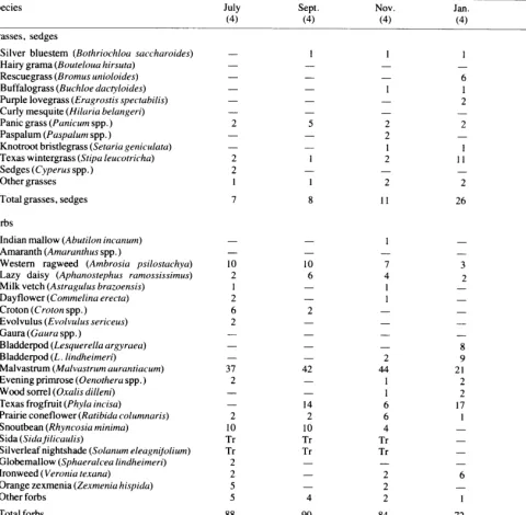
Available Soil Water (% by vol.)
SUMMER 1974
SPRING 1973
25-
-z u
x z 0,50- 0
75-
Argl
Bare / loo- 6.5 z’
:
I_
/ / I ‘-.5.0 - 5.0 profile
tunglehead, Trca= Arizona cottontop). Total available water (cm) in the IOO-cm projile shown across bottom.
Cm available water in 100 cm Fig. 1. Comparison between spring 1973 and summer 1974 in avuiluble soil
wuter ut maximum recharge at bare soil andplunt locutions ut site 4 (Arg’ = Santa Rita threeawn, Arte = spidergrass, Boer = black grama, Heco =
Table 3. Spring 1973 soil water losses (% by volume) following good winter recharge; averaged over all depths showing recharge.
Species
Starting available water Total loss
tefstl
t
% by volume’ CV
Loss per Profile depth
% by volume’ test’ CV day (cm)
Grasses
Santa Rita threeawn 8.0 & 0.2 9.4
Black grama 9.3 & 0.4 17.3
Spidergrass 9.8 + 0.8 27.1
Tanglehead 11.5 -+ 0.4 ** 13.2
Arizona cottontop 9.7 ? 0.6 24.2
Bare soil 8.52 0.6 20.1
Slender grarna 9.3 * 0.3 14.9
Bare soil 8.5 ? 0.5 16.8
Bush muhly 9.9 ‘-r- 0.6 24.1
Bare soil 8.7 ? 0.8 26.4
Lehmann lovegrass (site 2) 10.0 + 0.3 ** 12.3
Bare soil 8.0 2 0.6 19.5
Lehmannlovegrass (site 3) 14.0 -+ 1.0 * 17.4
Bare soil 9.7 ‘-’ 1.5 38.8
Buffelgrass (pit) 12.9 ? 0.7 16.7
Buffelgrass (flat) 11.2 !I 0.5 12.3
Bare soil (Rat) 8.4 t 1.6 59.6
6.7 + 0.2 7.8 2 0.4 8.0 + 0.4 9.0 2 0.3 8.2 & 0.4 4.6 + 0.7
** ** ** ** **
9.0 0.066 100
25.0 0.083 100
17.7 0.094 100
10.3 0.092 100
21.7 0.085 100
41.6 0.048 100
16.0 0.088 19.2 0.061
100 100 100 100
25.5 0.083
27.0 0.060
13.5 0.065 100
21.0 0.032 100
20.6 0.141 75
65.3 0.051 75
22.0 0.120 125
14.6 0.116 100
70.2 0.076 125
8.2 + 0.3 6.4 + 0.4 8.5 + 0.5 7.1 2 0.7 8.7 ? 0.3 3.6 + 0.3 12.3 + 1.0 6.1 ? 1.6 10.8 + 0.8 9.6 + 0.5 7.2 I? 1.6
**
**
**
*
Shrubs
False-mesquite 9.0 IT 1.1 29.4 7.7 + 1.2
Bare soil 9.7 + 1.5 38.8 6.1 ? 1.6
Fourwing saltbush (swale) 10.8 + 1.6 33.0 8.9 t 1.8
Fourwing saltbush (slope) 7.3 4 1.2 64.2 5.9 ?I 1.2
Bare soil (slope) 11.1 ? 1.8 44.6 9.4 ? 1.8
Creosotebush (swale) 11.7 + 1.0 20.1 10.8 2 1.0
Creosotebush (slope) 3.8 ? 0.9 ** 92.6 2.8 + 0.8
Bare soil (slope) 9.0 -+ 1.9 65.9 7.3 ? 1.6
39.4 0.104 75
65.3 0.05 1 75
44.4 0.108 125
81.2 0.088 125
53.6 0.106 100
21.2 0.119 125
115.0 0.050 125
71.6 0.094 125
**
’ Means 2 one standard error
2 **P ~0.01, *P<O.O5, + P<O. 10, for differences between soil with plants and bare soil
Table 4. Summer 1974 soil water losses (% by volume), averaged over all depths showing recharge.
Species
Starting available water Total loss
t t Loss per Profile depth
% by volume’ test’ CV” % by volume’ test” CVj day (cm)
Grasses
Santa Rita threeawn Black grama Spidergrass Tanglehead Arizona cottontop Bare soil Slender grarna Bare soil Bush muhly Bare soil
Lehmann lovegrass (site 2) Bare soil
Lehmann lovegrass (site 3) Bare soil
Buffelgrass Buffelgrass Bare soil Shrubs
False-mesquite Bare soil
(pit) (flat) (flat)
5.0 +- 0.9 5.1 2 0.8 5.0 + 1.0 9.5 + 0.8 5.8 -+ 0.8 3.0 -+ 1.0 6.8 +- 1.3 3.8 IL 1.1
6.0 -+ 1.1 4.4 r 1.4 10.2 +- 0.2 8.4 ? 0.5 13.0 -+ 1.6 3.0 +- 1.4 12.0 ZZ 1.0 8.0 ? 1.3 1.8 2 0.6
Fourwing saltbush (swale) Fourwing saltbush (slope) Bare soil
3.1 -t 1.2 4.52 1.7 14.5 -t 1.9 4.7 -+ 1.4 1.9 -+ 0.7 Creosotebush (swale) 6.6 2 2.6 Bare soil (slope) 1.7 +0.4 Creosotebush (slope) 4.6 +- 1.8 Bare soil (slope) 3.7 -+ 0.4
** * + ** ** ** ** ** + * 65.1 62.3 65.4 29.1 52.3 94.7 52.9 83.0 61.5 79.4 7.1 15.9 29.6 118.7 26.4 44.5 94.8 78.6 77.4 28.6 84.0 100.4 78.6 75.7 69.1 15.3 ’ Means one standard
z **P<O.Ol. *P<O.O5, fP<O. 10. for differences between soil with plants and bare soil
4.1 ?I 0.8 4.2 2 0.7 4.0 +- 0.9 8.4 + 0.9 4.9 2 0.7 2.0 ? 0.7 6.1 ? 1.2 2.5 ? 0.8 5.0 ? 1.0 2.8 21.2 8.0 + 0.2 4.1 20.1 11.4 ?I 1.7
1.6 -+ 0.9 10.6 + 0.9 7.5 + 1.2 0.5 _+ 0.4
1.9 t 1.2 2.4 k 1.2 12.0 _+ 2.4 3.6 2 1.3 0.6 t 0.5 6.1 k 2.6 0.6 f 0.4 3.4 2 2.1 2.3 k 0.2
.i Coefficient of variation (%)
relatively dense colony with a good cover of litter. Recharge of soils occupied by the other four species fell between the extremes of bare soil and soil with tanglehead, but with sharply lower recharge with increasing depth. These plants were in the more open stands where much of the soil was exposed, and high surface runoff in the summer would be expected.
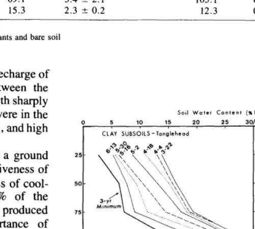
So,1 water Content (rbyvol)
CLAY SUBSOILS-Tanglehead
15 20
SANDY SUBSOILS-Santa Rnta threeawn
The practical implication of these results is that a ground cover of plants and litter greatly increases the effectiveness of summer precipitation, but increases the effectiveness of cool- season precipitation only moderately. Since 90% of the perennial grass forage on southern Arizona ranges is produced from summer rainfall (Culley 1943) the importance of maintaining an adequate ground cover of forage plants and litter is apparent. In other words, adequate ground cover is not essential for the production of winter-spring annuals, but it is necessary for high yields of warm-season perennial grasses.
v
Water-holding capacities of the soils were strongly affected by differences in texture, primarily of the subsoils, as would be expected. Amounts of water available at the start of the 1973 spring deletion period for finer subsoils ranged from 10.8 to 14.0% compared to the 8 to 10% for predominantly sandy or mixed subsoils. Finer subsoils were those associated with tanglehead, Lehmann lovegrass at site 3, the pit position buffelgrass, and the swale position four-wing saltbush and creosotebush (Table 4). The contrast between high water- holding capacity of clay subsoils occupied by tanglehead and sandy subsoils occupied by Santa Rita threeawn is particularly
Fig. 2. Maximum recharge on March 22,1973,jollowing above-average winter
precipitation, as injluenced by texture oj the subsoil, and subsequent dep-
letion patterns during the dry spring f3-year minimum = lower limit ojavail- able water).
12 JOURNAL OF RANGE MANAGEMENT33(1), January 1980
+ + ** * * ** ** ** ** ** * **
71.8 0.093 100
70.1 0.080 100
78.0 0.087 100
36.8 0.157 125
58.2 0.094 100
96.7 0.070 100
54.2 0.160 100
90.7 0.057 100
69.5 0.105 75
108.9 0.065 75
12.4 0.123 100
10.0 0.069 100
36.0 0.220 75
138.0 0.028 75
26.8 0.220 125
43.8 0.108 100
227.9 0.007 100
123.2 0.053 50
98.3 0.042 50
43.7 0.177 125
103.5 0.104 11
213.8 0.012 100
84.6 0.074 100
186.1 0.049 100
105.1 0.104 25
noticeable in both spring and summer at site 4 (Figs. 1 and 2). Clay content of the subsoil with tanglehead increased with increasing depth, as indicated by the rapidly increasing 3-year minimum water content (Fig. 2), whereas the relatively low, but constant, 3-year minimums at all depths for the subsoil with Santa Rita threeawn indicate relatively uniform sandy textures and similar water-holding capacities throughout the profile. Generally deeper penetration of water due primarily to increased duration of surface flow or ponding made large volumes of available water for plants at the pit and swale positions (Table 4 and 5). Recharge at the swale-position fourwing saltbush plants, for example, reached 150 cm in the summer of 1974 (Fig. 3), with 15.9 cm of available water at maximum recharge (July 25) in the 150-cm profile, compared to penetration to about 75 cm and only 4.4 cm available water at the slope-position plants (July 10). Available water at bare soil locations (August 21) was 3.2 cm with moisture penetrating to only about 25 cm. The relative advantages of pit and swale positions are more marked in wetter than in drier seasons because the amounts of runoff in drier seasons are smaller and less frequent.
Available Soil Water (% by vol.)
5
z
0
h ‘\
IOY 200- ‘, , 1
III / :I I I
!i
1 1 I250-:I 1 !
,I II :I Ii I!
300 -’ ‘6
Fig. 3. Soil water profiles at the time of maximum recharge at 25 cm (July 10, 1974) and during the following depletion period jo r soil with jourwing salt- bush plant in a swale, jor plants on an adjacent slope, and jor bare soil.
Depletion Characteristics
The two major periods of soil water depletion in southern Arizona are: (1) the spring growing period, when plants use accumulated cool-season moisture, and (2) the summer growing period, when plants use current precipitation. Depletion patterns differ between spring and summer. Spring depletion starts slowly as warming spring temperatures permit plant
growth to begin, increases to a relatively constant high rate during the main period of spring growth (usually 4 to 8 weeks), then tapers off as soil water is depleted. In summer temperatures are high, plant growth is limited by the moisture supply, and evaporation is rapid.
One broad general result of the study was to show that evapotranspiration usually removed all available soil water by the end of each depletion period. This agrees with the view of W ilm ( 1962) that in arid areas all soil water is lost to evaporation or transpiration whether vegetation is present or not. Con- sequently, differences in observed evaporation losses between seasons and between kinds and amounts of vegetation were due largely to differences in the amount of soil water available at the start of the depletion periods. For example, following a winter of high recharge, starting available water in the spring of 1973 ranged from 3.8 to 14% and total loss from 2.8 to 12.3% (Table 3). During the relatively wet summer of 1974, initial available water varied from 1.7 to 14.5% and losses from 0.5 to 12.0% (Table 4). Regressions, derived from Tables 4 and 5, indicate that on vegetated plots the initial soil water content was associated with 97% of the variation in loss of winter soil water and with 98% of the summer loss. Comparable values for bare plots were 49% for winter moisture and 89% for summer. The higher correlation in summer is probably due to the fact that available summer moisture in bare soil usually is confined to the upper 25 cm of soil, where it evaporates more rapidly than moisture from deeper layers that contain much of the accumulated cool-season moisture.
Total water losses from soil with plants were significantly higher than those from bare soil at most grass sites. Fewer such differences were significant at shrub sites because of fewer plants and higher standard errors (Tables 3 and 4). Deviations of soil water depletion rates from regression indicate that slender grama, buffelgrass, and tanglehead extracted water faster than other species during the wet summer of 1974, and that Lehmann lovegrass extracted water more slowly.
Depths to which the soil was recharged were about the same for grasses in summer as in spring; but depths of recharge at shrub locations were only a little more than half as deep in the summer as in the spring, because the finer textured relatively bare soils at the shrub locations had lower infiltration rates and they sealed over quickly during summer thunderstorms.
Bare soil lost less water than vegetated soils in both seasons- one-fifth less in spring, but two-thirds less in summer. This difference between seasons was particularly marked for bare locations with clayey subsoils, which recharge very poorly in summer and thus had less water available (Tables 3 and 4). In all seasons, losses from bare soil tended to be slower and at more uniform rates than from vegetated soil. For example, ET loss from clay soil with Lehmann lovegrass plants at site 3
Table 5. Evapotranspiration losses (cm) during wet and dry spring and summer depletion periods, by depths, averaged over all species at all locations.
Depth 25 50 75 100 125 150
Total Available at start
Wet spring 1973 Wet summer 1974 Dry spring 1974 Dry summer 1973
Plants Bare Plants Bare Plants Bare Plants Bare
2.34 2.32 2.08 0.92 1.48 1.57 0.79 1.03
2.13 1.98 1.65 0.41 0.35 0.26 0.38 0.62
1.98 1.53 1.15 0.19 0.03 0.14 0.33 0.59
1.57 0.86 0.66 0.17 0.39 0.48
0.18 0.15 0.10 0.01 0.18 0.16
0.04 0.07 0.15
8.24 6.91 5.64 1.70 1.86 1.97 2.07 3.03
essentially exhausted available moisture from the upper 75 cm of soil within 2 weeks after maximum recharge in the summer. Bare soil lost water at much lower rates for 6 weeks but mainly from the upper 25 cm layer because deeper soil layers were not wet. The period of rapid soil water depletion in the summer of 1974 varied from 2 to 6 weeks among species and depths. Similar rapid extraction of soil water during the summer was reported for Arizona cottontop and burroweed in an earlier study (Cable 1969).
The ability of semidesert plants to extract water rapidly when it is available is crucial to their survival because soil water that is not picked up quickly by plant roots is soon lost by evaporation.
Subsoil Texture Effects
Differences in subsoil texture strongly affected soil water- holding capacities and amounts of soil water available to plants, as would be expected. At site 4, 22 soil water sampling tubes were installed on an apparently uniform area of about 25-meter radius to sample soil water changes for five perennial grass species and bare soil. Subsoil textures varied from loamy sand to gravelly clay; available soil water at maximum recharge varied from 8.3% by volume in the upper 100 cm of sandy loams and loamy sands at the Santa Rita threeawn plants, to 12.8% in the gravelly clay subsoils at the tanglehead plants. For the other three species, maximum available water varied from 10.0 to 10.3% by volume. These values of maximum available water agree well with those reported for similar soil textures for other environmental situations by Lassen et al. (1952) and Hoover (1962). These data show that subsoil textures, and thus relative amounts of available water, can vary considerably within a relatively small area and suggest that the distribution of species on such an area is strongly affected by soil conditions. Some species apparently are more adaptable than others to soils of varying texture and water-holding capacity. The subsoil- species distribution relationships at site 4 and depletion characteristics during the spring depletion period of 1973 (Fig. 2) show that: (1) clay subsoils, as expected, held the most available soil water, sandy subsoils the least, and the variable subsoils intermediate amounts; (2) ET losses from bare soil were less than from soil with plants and decreased uniformly with increasing depth; (3) in soil with plants, water was extracted most rapidly at the shallower depths early in the depletion period and at successively greater depths as the period advanced, which probably indicates decreasing root densities with increasing depth (Hillel 197 1); (4) by June, available soil water was reduced to from 2 to 3% for the three grasses, but the bare soil held noticeably more available water because of lower rates of loss; and (5) the relatively uniform total depletion within the upper 100 cm of soil for each species indicates that the root systems of all three reach to at least 100 cm. Limited data from 125 and 150 cm indicate that the taller grasses extracted some water at 125 cm but little or none at 150 cm.
Dry-Season Depletion
In growing periods with deficient precipitation, such as the spring of 1974 and the summer of 1973, available soil water supplies were very low. Recharge usually was limited mainly to the upper 25 cm or so of soil. For example, in the dry spring of 1974, 80% of the total ET losses from both bare soil and soil with plants came from the upper 25 cm, indicating very little recharge below 25 cm (Table 5). In the dry summer of 1973, however, small amounts of soil water were present throughout the profile as carryover from the preceding unusually wet winter. Carryover moisture was significantly greater (PcO.01) for bare soil than for plant locations. Depletion patterns during
droughty growing periods appear to be similar on bare and vegetated areas. During such periods, perennial grasses use water that would be lost by evaporation if the plants were not present, since they produce some green foliage even in the driest seasons. After prolonged dry periods (e.g., summer 1973), essentially no available water was left in the soil. Available water was reduced to between 1 and 2% by volume at all depths by the end of most depletion periods (Table 6).
Management Implications
The productivity of semidesert ranges depends on the supply and disposition of available soil water. The supply of soil water depends on: (1) precipitation amounts, (2) water holding capacity of the soil, as determined by soil depth and texture, and (3) surface condition of the soil, as it affects infiltration and surface runoff. Precipitation and soil characteristics set the upper limits on the amount of available water and are not amenable to control. Infiltration rates, however, can be influenced considerably by manipulating the vegetation cover. Vegetation can increase infiltration not only by protecting the surface from the puddling actions of raindrops, but also by the action of roots in maintaining a friable open soil, more receptive to the infiltration and downward movement of water. The importance of vegetation in promoting infiltration was particularly evident in the wet summer 1974, when 7.3 cm of water was available at maximum recharge in soil with plants, and only 3.3 cm at bare locations (Table 5).
Once in the soil, available water on semidesert ranges either evaporates or is used by plants. Plants and litter shade the soil, thereby reducing the temperature and air movement at the soil surface and retarding the rate of evaporation. The only way to prevent the eventual loss of all soil water to evaporation is to use part of the moisture for plant growth. A plant can only use moisture that is within reach of its roots; consequently, all moisture in soil that is not occupied by plant roots will be lost by evaporation. Evaporation also takes a part of the moisture from soil that is occupied by plant roots. Plant growth, therefore, is made during relatively short periods between soil wettings and times when evaporation and transpiration have removed all readily available water. Evaporation losses are minimized and forage production is maximized when the roots of forage plants occupy as much of the soil profile as possible and when there is enough litter to cover the soil surface between plants.
A major objective in the management of semidesert range is to get maximum use of precipitation. This requires getting as much water as possible into the soil and using that water as rapidly as possible for plant growth-before it evaporates. The most effective means for doing this is by maintaining a dense ground cover of valuable perennial grasses. Most native semidesert grasses are primarily summer growers. Water losses to runoff and evaporation are especially critical for such grasses because these losses are greatest during the summer rainy season.
Summary and Conclusions
Soil water recharged to greater depths from cool-season rainfall than from summer rainfall and lasted longer. Bare soil recharged almost as well as vegetated soil in winter; but summer recharge of bare soil was only one-third that of vegetated soil, and there was little recharge below 25 cm.
Well-vegetated soil recharged about as well in summer as in winter. In the summer of 1974, more than twice as much water was available at vegetated locations as in bare soil. Perennial