Combining Faraday Tomography and Wavelet Analysis

(1)

Combining Faraday Tomography and Wavelet

Analysis

Dmitry Sokoloff1*, Rainer Beck3, Anton Chupin2,5 ID_{, Peter Frick}2,5_{, George Heald}4_{, Rodion} Stepanov2ID

1 _{Department of Physics, Moscow University, 119992 Moscow, Russia}

2 _{Institute of Continuous Media Mechanics, Korolyov str. 1, 614061 Perm, Russia} 3 _{MPI für Radioastronomie, Auf dem Hügel 69, 53121 Bonn, Germany}

4 _{CSIRO Astronomy and Space Science, 26 Dick Perry Avenue, Kensington, WA 6151, Australia} 5 _{Perm State National Research University, Perm, Russia}

* Correspondence: [email protected]; Tel.: +x-xxx-xxx-xxxx

Abstract: We present an idea how to use long-wavelength multi-wavelength radio continuum observations of spiral galaxies to isolate magnetic structures which were previously accessible from short-wavelength observations only. The approach is based on the RM-synthesis and 2D continuous wavelet transform. Wavelet analysis helps to recognize a configuration of small-scale structures which are produced by Faraday dispersion. We find that these structures can trace galactic magnetic

arms for the case of the galaxy NGC 6946 observed atλ=17÷22 cm. We support this interpretation

by an analysis of a synthetic observation obtained using a realistic model of a galactic magnetic field.

Keywords:galactic magnetic field; RM-synthesis; Faraday depolarization; wavelet analysis

1. Introduction

The main bulk of contemporary knowledge concerning magnetic field configurations in spiral galaxies is obtained based on observations performed at a few wavelengths only. Modern progress in observational techniques allows us to observe galaxies at dozens and hundreds of wavelengths. It is however important to learn how to use this new tool. Some problems which arise in this way

are illustrated at Fig.1. The left panel gives the linearly polarized intensity distribution of NGC

6946 atλ =6 cm from Becket al.[1]. Magnetic spiral arms are clearly seen. Magnetic arms can be

important because they possibly are magnetic reconnection regions [2] or may also be products of

dynamo action [3]. However their origin remains unclear [4]. The middle panel shows the polarized

intensity distribution obtained aroundλ=20 cm in the modern multi-wavelength observations in the

spectral range from 17 to 22 cm. The plot looks almost empty. It happens because of two reasons. On one hand, it is impractical to observe at each spectral channel as long as it was done in observations performed at just one wavelength. On the other hand, depolarization effects by Faraday rotation are

much more pronounced at longer wavelengths rather atλ=6 cm.

One can try resolve the problem in two ways. Firstly, it is possible to sum polarized intensities over

all channels in the rangeλ=17÷22 cm to emulate single-wavelength observations atλ≈20 cm. This

option, however, does not look attractive because it means that we emulate old-fashion results using modern observational technique. Another option is to use RM-synthesis which involves processing data at many wavelengths. Reconstruction of magnetic field even along a single line of the sight

remains a challenging problem [5]. 3D RM-cube data (i.e. maps of polarized intensity at many

wavelengths) can be processed in various ways. A straightforward approach is to pick up maximum

values of Faraday spectra (i.e. the distribution of polarized intensity as a function of Faraday depth) [6].

The resulting distribution ofFmaxis shown in Figure1(c). The signals are much stronger than those

shown in Figure1(b). However, we do not see here the narrow magnetic arms visible in Figure1(a)

because they are suppressed by Faraday depolarization effects atλ=17÷22 cm.

(2)

(a) (b) (c)

34′₃₀″ 34′_37.50" 34′₄₅″ 34′_52.50" 35′₀″ 35′_7.50" 60◦₄′ 60◦₆′ 60◦8′ 60◦₁₀′ 60◦₁₂′ 60◦14′

Right ascension(-20h)

Declination

0.6 1.3 2. 2.7 3.4

×102

33′₄₅″ 34′₀″ 34′₁₅″ 34′₃₀″ 34′₄₅″ 35′₀″ 35′₁₅″ 35′₃₀″ 35′₄₅″ 59◦₅₂′ 59◦56′ 60◦₀′ 60◦₄′ 60◦8′ 60◦12′ 60◦₁₆′ 60◦₂₀′ 60◦24′

Declination

0.6 1.8 3. 4.2 5.4

×103

34′₁₅″

34′₃₀″

34′₄₅″

35′₀″

35′₁₅″

35′₃₀″

60◦₀′

60◦₄′

60◦8′

60◦₁₂′

60◦16′

Declination

0.4 1. 1.6 2.2 2.8

Figure 1.(a) Polarized intensity distribution in NGC 6946 atλ=6, (b)λ=20 cm, and (c) peak Faraday

spectraFmaxsynthesised fromλ∈17÷22cm.

We face a difficult choice: to postpone multi-wavelength observations of magnetic arms in spiral galaxies until the forthcoming SKA telescope will be ready for observations in its full extent or to suggest a method which allows to recover magnetic arms from the available multi-wavelength data taken at long wavelengths. The second way looks more attractive. The desired method is described by

Chupinet al.[7]. Technical details of the method are rather bulky. It is why here we present the idea of

the method in a compressed form and illustrate it by an example of the NGC 6946 data obtained by

Healdet al.[6] atλ=17÷22 cm (Section2) and by an artificial example (Section3).

2. Idea of the method applied to the NGC 6946 data

The method under discussion [7] departs from the point that polarized observations performed at

the wavelengthλ∗are most informative for magnetic structures of the scalel∗for whichλ2RM∝λBnel

is comparable withπ. Indeed, contribution from the structures withl l∗is strongly depolarized

due to Faraday rotation while Faraday rotation from the structures withl l∗ is too weak to be

useful. It means that using observations atλ1=20 cm instead of that ones atλ2=6 cm we deal with

magnetic structures that are an order of magnitudes smaller ((λ2/λ1)2≈10). In other words, instead

of detecting magnetic arms by large scales we have to do it by small-scale structures which arise by tangling and randomizing of large-scale structures, in addition to small-scale structures by small-scale turbulent magnetic fields predicted by dynamo theory.

Realization of the idea suggested in [7] is based on wavelet technique. Wavelet functions are

used for an analysis of spatial and temporal data, also in astrophysics[8]. The wavelet transform can

be used as an advance of RM-synthesis to structure analysis at different scales [9,10]. Here wavelets

are used as a spatial-scale filtering tool. We decompose all all maps of polarized intensity at a given

Faraday depth by wavelets of various scales (wl) and then find a peak intensitywmaxalong each line

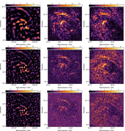
of sight. Results for various scaleslmeasured in arcseconds are shown in the middle row of Figure2.

We recognize small-scale structures at the scale ˆl=16 arcsec that are ordered as arm-like structures.

The structures at smaller and larger scales are less pronounced. In other words, we traced the structure

of magnetic arms known fromλ1 =6 cm using the data obtained atλ2 =20 cm. In a comparison

the result of wavelet decomposition of polarized intensity at 6 cm (left row of Figure2) and the peak

Faraday spectraFmax(right row of Figure2) are much noisier. The technical details of the method are

(3)

34'52.50" 35'0"

35'7.50"

60°4'

60°6'

60°8'

60°10'

Declination

0. 1.5 3. 4.5 6.

×102

34′45″

35′0″

35′15″

60◦4′

60◦8′

60◦12′

Declination

0.4 1.2 2. 2.8 3.6

34′45″

35′0″

35′15″

60◦4′

60◦8′

60◦12′

Declination

0. 1. 2. 3. 4.

34'52.50" 35'0" 35'7.50" 60°4' 60°6' 60°8' 60°10'

Declination

0.2 1.1 2. 2.9 3.8

×102

34′45″

35′0″

35′15″

60◦4′

60◦8′

60◦12′

Declination

0.4 1.2 2. 2.8 3.6

34′45″

35′0″

35′15″

60◦4′

60◦8′

60◦12′

Declination

0.2 1.1 2. 2.9 3.8

34'52.50" 35'0"

35'7.50"

60°4'

60°6'

60°8'

60°10'

Declination

0.2 0.6 1. 1.4

×102

34′45″

35′0″

35′15″

60◦4′

60◦8′

60◦12′

Declination

0.2 0.6 1. 1.4 1.8

34′45″

35′0″

35′15″

60◦4′

60◦8′

60◦12′

Declination

0. 1. 2. 3. 4.

Figure 2.Wavelet coefficients of the scales 32, 16, 8 arcsec: (leftcolumn) for PI at 6 cm, (middlecolumn)

wmax_{, (right}_{column) for}_Fmax_.

3. Synthetic data analysis

We constrain a model magnetic field to demonstrate qualitatively the applicability of our approach

and to support an interpretation of the results. The galactic magnetic field~Bg is modelled as a

superposition of a large-scale component~Band a small-scale turbulent component~b:

~

Bg(~r) =~B(~r) +~b(~r), (1)

where~ris the radius vector in the cylindric coordinate system (r,φ,z). The regular part of magnetic

field is assumed to be of bisymmetric form with two reversals along azimuthal angle:

B(r,φ,z) =B0cos

m

lnr

tanp −φ+φ0

tanh r r0 exp ( − r R0 2) exp ( − z h0 2) , (2)

whereB0is the field amplitude (strength) andφ0is the azimuthal phase of the modem,pis a pitch

(4)

term is introduced to suppress a peculiarity near axis at characteristic radiusr0[11]. Then components of regular magnetic field are evaluated by

Br(r,φ,z) = B(r,φ,z)sinp, (3)

Bφ(r,φ,z) = B(r,φ,z)cosp, (4)

∂zBz(r,φ,z)) = −r−1 (∂r(rBr(r,φ,z)) +∂φBφ(r,φ,z)

, (5)

where a latter relation is a result of the incompressibility condition.

The turbulent magnetic field is considered as a divergence-free, random fluctuating field with the

given energy spectraΨand Gaussian spatial distribution with the radiusRtand the vertical scaleht:

~_b(r_,_φ_,_{z) =}_b_0Ψ_(r_,_φ_,_z)_exp

(

−

r Rt

2)

exp

(

−

z ht

2)

, (6)

whereb0is the strength of the turbulent field. The spectral property of the random functionΨare

specified as follows:

|_Ψˆ(~k)|2₌ (

(k/k0)α, k>k0

(k/k0)β, k<k0.

(7)

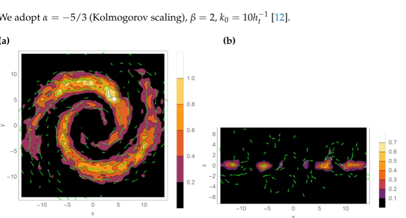
We adoptα=−5/3 (Kolmogorov scaling),β=2,k0=10h−1t [12].

(a) (b)

Figure 3.Distribution of model magnetic field: (a) in central horizontal galactic plane, (b) in central vertical plane.

Figure3shows the distribution of galactic magnetic field in three-dimensional numerical domain

14×14×14 kpc3 with resolution 0.4 kpc for a particular choice of parameters: m = 1, p = π/12,

h0=1 kpc,R0=14 kpc,r0=4 kpc,Rt=20 kpc,ht =4 kpc andB0=b0=1. Thermal electron and

cosmic rays densities are adjusted to get qualitative correspondence with the observation. We use simulated magnetic field to calculate an artificial maps of polarized intensity and Fadaray rotation for

λin the observed range from 17 to 22 cm. Then synthetic RM-cube is analysed by the same approach

as NGC 6946 data in the Section2.

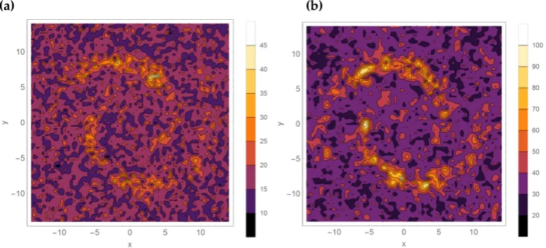
For the case of zero-noise contribution in polarized intensity the distribution of Fmax (see

Figures4(a)) is slightly affected by Faraday depolarization. We note the result does not differ from

the initial distribution in Figure3(a) because the rotation measures are rather moderate (a few tens

(5)

emission is considerably scattered over the Faraday depths so that small-scale structures appear in

distribution ofwmax(see Figures4(b)). Nevertheless the large-scale structure of galactic magnetic arm

is well traced bywmax.

(a) (b)

Figure 4.Distributions for a model which consists of large scales and small scales (no noise): (a)Fmax, (b)wmax.

The situation is substantially changed in the case if a white noise of levelS/N =20 is added

to the ideal observations. Figure5shows resulting distribution ofFmaxandwmaxin the presence of

the noise. The galactic signal inFmax_{representation is getting much weaker. At the same time the}

distribution ofwmaxreveals the magnetic arms with a patchy structure.

(a) (b)

Figure 5.Distributions for a model which consists of large scales, small scales and noise: (a)Fmax, (b)

wmax.

4. Discussion

(6)

a galactic magnetic field. The above results demonstrate that the method can be helpful in practice especially in the case of noisy polarization data at an individual wavelength. However, we keep in mind that small-scale structures of a magnetic field may contribute in wavelet coefficients. Existence of such structures was a general expectation from dynamo theory but the previous methods do not allow isolating this. We note that wavelet technique can be successfully combined with modern approaches

like the Faraday tomography [13] and the method based on the synchrotron derivative polarization

gradients [14]. Then one can probe the local interstellar medium in the Galactic foreground towards

some galaxies [15]. Our model of galactic magnetic field may be also useful for validation of processing

results.

Author Contributions: The idea of the method presented here belongs to R.S. and A.Ch., P.F. embedded the method in the general framework of wavelet methods, D.S. is responsible for the link with dynamo studies, R.B. elaborated the link with classical RM-synthesis, the observational data exploited was obtained by G.H.

Acknowledgments: Numerical simulations were performed on the supercomputers URAN and TRITON of Russian Academy of Science, Ural Branch. D.S. is grateful for RFBR project under grant 18-02-00085 and the grant 18-1-1-77-1 from Basis Foundation.

Conflicts of Interest:The authors declare no conflict of interest.

Abbreviations

The following abbreviations are used in this manuscript:

VLA Very Large Array

LOFAR European Low Frequency Array SKA Square Kilometre Array RM Rotation measure

References

1. Beck, R.; Frick, P.; Stepanov, R.; Sokoloff, D. Recognizing magnetic structures by present and future radio telescopes with Faraday rotation measure synthesis. Astron. Astrophys. 2012, 543, A113, [arXiv:astro-ph.IM/1204.5694]. doi:10.1051/0004-6361/201219094.

2. We ˙zgowiec, M.; Ehle, M.; Beck, R. Hot gas and magnetic arms of NGC 6946: Indications for reconnection heating?Astron. Astrophys.2016,585, A3,[1603.00715]. doi:10.1051/0004-6361/201526833.

3. Beck, R. Magnetic fields in spiral galaxies. The Astronomy and Astrophysics Review2015,24, 4,[1509.04522]. doi:10.1007/s00159-015-0084-4.

4. Chamandy, L.; Shukurov, A.; Subramanian, K. Magnetic spiral arms and galactic outflows. Mon. Not. R.

Astron. Soc.2015,446, L6–L10,[arXiv:astro-ph.GA/1408.3937]. doi:10.1093/mnrasl/slu156.

5. Sun, X.H.; Rudnick, L.; Akahori, T.; Anderson, C.S.; Bell, M.R.; Bray, J.D.; Farnes, J.S.; Ideguchi, S.; Kumazaki, K.; O’Brien, T.; O’Sullivan, S.P.; Scaife, A.M.M.; Stepanov, R.; Stil, J.; Takahashi, K.; van Weeren, R.J.; Wolleben, M. Comparison of Algorithms for Determination of Rotation Measure and Faraday Structure. I. 1100-1400 MHz. Astron. J.2015, 149, 60, [arXiv:astro-ph.IM/1409.4151]. doi:10.1088/0004-6256/149/2/60.

6. Heald, G.; Braun, R.; Edmonds, R. The Westerbork SINGS survey. II Polarization, Faraday rotation, and magnetic fields. Astron. Astrophys. 2009,503, 409–435,[arXiv:astro-ph.GA/0905.3995]. doi:10.1051/0004-6361/200912240.

7. Chupin, A.; Beck, R.; Frick, P.; Heald, G.; Sokoloff, D.; Stepanov, R. Magnetic arms of NGC6946 traced in the Faraday cubes at low radio frequencies. Astron. Nachr.2018,[1808.05456]. doi:10.1002/asna.201813488. 8. Schwinn, J.; Baugh, C.M.; Jauzac, M.; Bartelmann, M.; Eckert, D. Uncovering substructure with wavelets:proof of concept using Abell 2744. Mon. Not. R. Astron. Soc. 2018, p. 2446. doi:10.1093/mnras/sty2566.

9. Frick, P.; Sokoloff, D.; Stepanov, R.; Beck, R. Wavelet-based Faraday rotation measure synthesis. Mon. Not.

(7)

10. Frick, P.; Sokoloff, D.; Stepanov, R.; Beck, R. Faraday rotation measure synthesis for magnetic fields of galaxies. Mon. Not. R. Astron. Soc. 2011, 414, 2540–2549,[arXiv:astro-ph.GA/1102.4316]. doi:10.1111/j.1365-2966.2011.18571.x.

11. Stepanov, R.; Arshakian, T.G.; Beck, R.; Frick, P.; Krause, M. Magnetic field structures of galaxies derived from analysis of Faraday rotation measures, and perspectives for the SKA. Astronomy and Astrophysics

2008,480, 45–59,[0711.1267]. doi:10.1051/0004-6361:20078678.

12. Stepanov, R.; Shukurov, A.; Fletcher, A.; Beck, R.; La Porta, L.; Tabatabaei, F. An observational test for correlations between cosmic rays and magnetic fields. Mon. Not. R. Astron. Soc.2014,437, 2201–2216, [1205.0578].

13. Ferrière, K. Faraday tomography: a new, three-dimensional probe of the interstellar magnetic field. Journal

of Physics: Conference Series2016,767, 012006.

14. Lazarian, A.; Yuen, K.H. Gradients of Synchrotron Polarization: Tracing 3D Distribution of Magnetic Fields. The Astrophysical Journal2018,865, 59.

15. Van Eck, C.L.; Haverkorn, M.; Alves, M.I.R.; Beck, R.; de Bruyn, A.G.; Enßlin, T.; Farnes, J.S.; Ferrière, K.; Heald, G.; Horellou, C.; Horneffer, A.; Iacobelli, M.; Jeli´c, V.; Martí-Vidal, I.; Mulcahy, D.D.; Reich, W.; Röttgering, H.J.A.; Scaife, A.M.M.; Schnitzeler, D.H.F.M.; Sobey, C.; Sridhar, S.S. Faraday tomography of the local interstellar medium with LOFAR: Galactic foregrounds towards IC 342. Astron. Astrophys.2017,