Investigation of the velocity field downstream of a benchmark
vent using numerical simulation and hot-wire anemometry
Jan Sip1,*, Frantisek Lizal1, Jakub Elcner1, Jan Pokorny1, and Miroslav Jicha1
1Brno University of Technology, Faculty of Mechanical Engineering, Energy institute, Technicka 2896/2, Brno 616 69, Czech Republic
Abstract. The velocity field in the area behind the automotive vent was measured by hot-wire anenemometry in detail and intensity of turbulence was calculated. Numerical simulation of the same flow field was performed using Computational fluid dynamics in commecial software STAR-CCM+. Several turbulence models were tested and compared with Large Eddy Simulation. The influence of turbulence model on the results of air flow from the vent was investigated. The comparison of simulations and experimental results showed that most precise prediction of flow field was provided by Spalart-Allmaras model. Large eddy simulation did not provide results in quality that would compensate for the increased computing cost.
1 Introduction
The optimal conditions of the microclimate are mostly achieved by various air conditioning systems. The emphasis on purity and thermal comfort of indoor environment is increasing due to the fact that people nowadays spend more time indoors than in the past. Similar situation occurs in passenger car cabins, where optimal conditions of indoor air help to maintain active passenger’s safety. In order to achieve optimal conditions indoor of passenger cars, it is important to have detailed information about the air flow that is delivered into the cabin. Physical quantities describing this phenomenon are velocity, turbulent intensity and temperature.
The main experimental method used for research of air exhaled from cabin air vent is considered to be Particle Image Velocimetry (PIV) while Laser Doppler Anemometry (LDA) and Constant Temperature Anemometry (CTA) are classified between alternative methods. Nowadays, in time of rise of computer technology, computational fluid dynamics (CFD) methods become popular. Although CFD methods are very valuable for wide spectrum of results, its validation using experiments is necessary.
The research of car air vents is mostly focused on a complex view of airflow inside the car cabin. Yang [1] applied PIV method on a simplified model of passenger car cabin. Lee [2] performed experimental measurement using PIV method in a real cabin of a passenger car. He measured three vertical planes in total. The first plane led through the driver's seat, second divided the car in two halves and the last vertical plane led through the seat of co-driver. Significant differences in shape of airflow fields which led through the middle of both seats were explained by presence of driving wheel and brake. However, these components are often missing in idealized models of car cabins. Herwig [3] applied LDA method on
the experimental methods were coincident with appropriate configurations. The results also proved that influence of the insertion of the bend was significant.
2 Experimental stand
The experimental stand for the research of the car air vents contains fan which is powered by a laboratory power source (12 V). The airflow is calculated from the measured pressure loss on the orifice in the stabilisation section by EN ISO 5167. The experimental stand can be seen in fig. 1.
The benchmark air vent from a passenger car with five horizontal and five vertical lamellas which can be seen on fig. 2. was measured. Dimensions of the outlet cross section are 51 × 95 mm. 90 degrees bend was connected upstream of the air vent.
Fig. 1. The scheme of the experimental stand [10] 1 – suction pipe, 2 – temperature sensor Pt100, 3 – Fan, 4 – reduction, 5 – stabilisation section, 6 –pressure tap, 7 – orifice plate, 8 – reduction, 9 – pressure tap, 10 – bend, 11 – air vent, 12 – calibration unit, 13 – thermoanemometric probe, 14 – traverse system, 15 – control unit, 16 – CTA, 17 – PC, 18 – A/D converter, 19 – ambient sensor, 20 – Comet T7418, 21 – micromanometer, 22, 23 – pressure sensor, 24 – temperature measurement module
Fig. 2.Detail of measured air vent [10]
For the purpose of numerical calculations, an identical copy of the internal surfaces was created. This
geometry contains the stabilisation section, orifice plate, reduction and identical length of pipeline with 90 degrees’ bend, where the air vent is connected. The lamellas of the air vent were set accordingly to the experiment setting. Some simplifications were done on the inside surface of the air vent to achieve lower numerical cost. These simplifications do not affect the flow profile. Part of model geometry can be seen on fig. 3.
Fig. 3. The model geometry [10]
3 Experiment
The airflow of 90.7 m3/h was set during the experiment.
An exhaust of air into the free environment, i.e. without attached walls simulating real surrounding of passenger car, was considered.
The velocity field was measured using CTA method. The Dantec Streamline system – three-wire thermoanemometric probe 55R91 was used. A sampling rate of 2 kHz was set and 4000 samples were measured in each point.
The orientation of the coordinate system can be seen infig. 2. The origin of the coordinate system is located 20 mm downstream of the middle of the lower edge of the air vent. Probe shifting was realized using traverse system ISEL 3D. The distance between single measuring points was in the range of 4 – 6 mm and 36 vertical planes were measured in total. The first vertical plane was located in the origin of the coordinate system and it was parallel to the XZ plane of this system. The distance between the planes 1 to 21 was 10 mm, then the distance between planes was doubled.
The measurement uncertainty was determined by the procedure published in [11]. The measurement uncertainty for the representative airflow velocity before the air vent of value 10 m/s is 4.8 %. The main source of uncertainty is the process of calibration of the thermoanemometric probe, which cause 2 % of the uncertainty for the air speed of 10 m/s.
The Reynolds number is defined as
𝑅𝑒 =𝑢∙𝑑𝜈 (1)
where 𝑢 is the velocity magnitude (m/s), 𝑑 is the characteristic linear dimension (m) and 𝜈 is the kinematic viscosity (m2/s). The characteristic linear dimension is defined as
𝑑 =4∙𝑆𝜎 (2)
where 𝑆 is the area of the jet cross section (m2) and 𝜎 is the perimetr of cross section flow.
The Reynolds number was determined for the first measured plane downstream of the vent. The Reynolds number is 32,261 for this plane.
4 Numerical simulation
The numerical simulations were performed using commercial CFD solver Star-CCM+ v. 10.04 from CD-Adapco company. Several numerical approaches were tested to achieve results comparable with experiments. The approaches were: five turbulent models from unsteady Reynolds-Averaged Navier-Stokes (RANS) family and one Large Eddy Simulation (LES) approach. The following turbulence models were chosen from the RANS family:
Standard k-ε model (k-ε)
Standard k-ω model (k-ω)
SST k-ω model with low y+ (Low y+)
SST k-ω model with all y+ (All y+)
Spalart-Allmaras model (SPA)
Reynolds stress turbulence model (RST)
The Standard k-ε model was chosen for its robustness and good accuracy and is well suited to industrial-type applications, which obtain recirculation with heat transfer. The Standard k-ε model is a standard version of two-equation model that involves transport two-equations for turbulent kinetic energy and its dissipation rate. The Standard k-ω model differs from the Standard k-ε model in choice of the second turbulence variable. The Standard k-ω model is successful and mostly recommended for internal flow applications. The selected Standard k-ω model is the original version of Wilcox’s [12] model. Whereas the simulated phenomenon can be considered as a complex with combination of internal and external flow, it was decided to use Menter’s SST k-ω model [13], which combines advantages of k-ε model approach in free stream cases with k-ω model accuracy in near wall areas. This model was involved in two versions. With the low wall y+ approach, where the boundary layer is completely
modelled, and with the All y+ approach version, where the
solver decides if the boundary layer will be modelled or substituted with a function. This decision is dependent on value of y+ in a near wall cell. If the wall y+ is lower than
one, the boundary layer will be modelled. Otherwise, if the value of wall y+ is higher than 30, the boundary layer
will be substituted with a function. Although the Spalart-Allmaras was mainly developed for the aerospace industry, especially to solve flow past wing, its use can lead to good results in the area of air vent.
The LES approach was represented by the Wall-Adapting Local-Eddy Viscosity model which can be considered as the most evolved LES model. For the purpose of testing of these approaches, it was decided to use all the selected models with its default settings, though better values could be achieved by tuning of constants of particular model.
4.1 Mesh
Different computational meshes were generated for RANS and LES approaches. For RANS approach a
polyhedral mesh with three layers of prismatic layer which consist of 2.5 million of cells was created (fig. 4.).
This mesh was selected according to grid independence test performed on meshes of different sizes of the base element. The test was performed in a selected point and its results can be seen in fig. 5. For the purposes of incorporation of the low wall y+ approach into the
results a new version of mesh with different prismatic layer was created. This prismatic layer consists of ten rows and its near wall cell passes a condition of wall y+ < 1.
Fig. 4. Detail of the mesh used for RANS simulations [10]
For the LES approach, a mesh consisting of 16.8 million of cells with elements size that passes the Taylor microscale [14] condition was generated. The boundary area of the LES approach-based mesh was treated with a prismatic layer that consist ten rows of hexahedral layers with near wall cell size that passes low wall-y+ condition.
This allowed the full simulation of the boundary layer.
Fig. 5. The results of the grid independence test [10]
4.2 Physics
The case was solved as unsteady with the time step of 3.3×10⁻⁴ second for the RANS cases and 2×10⁻⁵ second
for the LES case. These values were selected to pass the condition of Courant number value equal to one. The
12 12,5 13 13,5 14
0 2 4 6
V
el
oc
ity
m
ag
ni
tud
e
[m
/s
]
velocity inlet boundary condition was prescribed at the inlet of the supply pipe. The uniform velocity profile with value of 6.02 m/s was defined according to experimental values. Outlet conditions were treated by enclosing the surroundings of the vent inside the box of sizes 650×400×400 mm, where pressure outlet with zero pressure resistance was prescribed.
The t
emporal discretization was performed by the implicit unsteady algorithm with the second-order temporal discretization scheme, and the convection term was discretized using the second-order upwind scheme. The initial part of the simulation was performed for 1 secondand then selected variables were averaged for 3 seconds to achieve mean values. Selected planes according to cross-sections measured during experiments were compared.5 RESULTS AND DISCUSSION
The results of experiment and CFD simulations are presented as velocity fields behind the examined benchmark air vent. These results were quantitatively compared on the basis of angles of direction of exhaled air and velocity profiles.
5.1 Direction angles
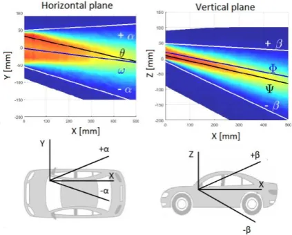
Direction angles were evaluated using the Matlab software (version R2018a). The border of the stream is determined as the point where the value of 10 % of the axial velocity is achieved [15]. The points defined as a border were linearly interpolated using least squares method. Direction angles are defined as deviation of these lines from axes of the car coordinate system [16]. This coordinate system and direction angles can be seen infig.
6.
Fig. 6. The coordinate system
The borders of streams are marked as ±α and ±β for the horizontal, resp. vertical plane. Spread of the stream is marked as δ and γ for horizontal, resp. vertical plane. The axis of stream is defined as arithmetic mean from the
spread of the stream and is marked as ω and ϕ for horizontal, resp. vertical plane. More accurate way to determine the axis of stream is interpolation of the maximal velocity from each plane. The axes of the stream defined with this method are marked as θ and ψ for horizontal, resp. vertical plane. The direction angles are in
fig. 7.
Fig. 7.The direction angles, CTA – horizontal plane [10]
Table 1. The direction angles for the horizontal plane [10]
Source +α [°] -α [°] δ [°] ω [°] θ [°]
CTA 2,21 -11,46 13,67 -4,63 -8,32
LES 6,23 -7,57 13,80 -0,67 -5,11
k-ω 5,55 -7,28 12,83 -0,87 -4,02
k-ε 5,08 -7,17 12,25 -1,05 -4,13
All y+ 5,43 -7,67 13,10 -1,12 -3,65
Low y+ 5,22 -7,34 12,56 -1,06 -5,75
RST 5,39 -8,41 13,80 -1,51 -1,54
SPA 5,96 -10,54 16,50 -2,29 -4,48
Table 2. The direction angles for the vertical plane [10]
Source +β [°] -β [°] γ [°] Φ [°] Ψ [°]
CTA -2,54 -20,67 23,21 -9,07 -10,26
LES 2,63 -20,05 22,68 -8,71 -7,04
k-ω 4,18 -17,11 21,29 -6,46 -8,24
k-ε -0,60 -18,36 18,96 -8,88 -10,41
All y+ 3,97 -17,43 21,40 -6,73 -8,22
Low y+ 2,58 -19,99 22,57 -8,71 -10,63
RST 1,49 -18,10 19,59 -8,31 -7,17
SPA 3,32 -20,82 24,14 -8,75 -10,44
The direction angles for the vertical plane obtained from experiments and numerical simulations were evaluated and their values can be seen in table 2. The top border of the stream in the vertical plane was most accurately estimated by the k-ε model of turbulence which was the only one to determine the negative value of the angle. The bottom border of the stream was most accurately predicted by the Spalart-Allmaras, Large Eddy Simulation and SST k-ω turbulence model with low wall y+ approach. All models predicted the value of -β with difference lesser than 1°. The axis of the stream calculated from its spread was predicted with deviance smaller than 1° by almost all of the models, except the Standard k-ω model and the SST k-ω model. The best results were achieved by the Standard k-ε model. The stream axis based on the maximal values of velocity was most accurately estimated by Standard k-ε model, Spalart-Allmaras and SST k-ω turbulence model with low wall y+ approach.
4.2 Velocity profiles
The commonly used method for comparison of measured and calculated velocity fields is to depict the velocity profiles. The velocity profile, which can be seen on fig. 8.
is located 22 mm above bottom edge of the air vent in distance of 60 mm in horizontal plane.
The highest peak of velocity is located on the left side of the air vent which is probably caused by presence of 90° bend upstream of the air vent. It can be seen that SST k-ω turbulence model with low wall y+ approach
significantly overrated the local maximum on the right side of the air vent. The drop in the velocity value can be seen in the axis of the velocity profile. This is probably caused by the presence of lamella in the axis of the air vent. This drop was not predicted by the Standard k-ω model and the SST k-ω model with all y+ approach. The
best match with the velocity profile measured during experiment was achieved by the Spalart-Allmaras and Standard k-ε model.
Fig. 8. The velocity profiles [10]
6 Conclusion
The comparison of results obtained during experiment and results calculated using numerical simulations revealed the turbulence models most suitable for predicting of airflow structures downstream of the passenger car air vent. The best match in the case of the direction angles provides the Spalart-Allmaras turbulence model. Good result was also provided by the Standard k-ε model and Large Eddy Simulations.
Because the purpose of this article was to compare several approaches on turbulent modelling (one or two-equations eddy viscosity models and large eddy simulation approach), modification of individual computational approaches was not considered for better reproducibility of achieved results. In future work it would be advisable to focus on choosing of specific modification and its impact on final results.
However, Large Eddy Simulation approach of turbulence modelling did not provide significantly better results than RANS models of turbulence to redeem the higher computational costs.
This fact is probably caused by two main reasons. Firstly, there were some uncertainties in the definition of boundary conditions. Velocity inlet was defined as uniform with insufficient length of the upstream pipeline for its developing. Secondly, the turbulence intensity on the velocity inlet was not measured and only default value was prescribed.
The results report large differences in prediction of the axis of the stream in the horizontal plane. The knowledge obtained during this study may be used for improving the reliability of analysis of the flow from the air vent using a smoke visualisation.
0 1 2 3 4 5 6 7 8 9
-100 -50
0 50
100
V
e
locity
[m
/s]
Y [mm]
k-epsilon k-omega
All y+ Low y+
experiment SPA
Acknowledgment
This work was supported by the internal Brno University of Technology research project Reg. No. FSI-S-17-4444.
References
1. J.H. Yang, S. Kato, H. Nagano, Journal of Visualization, 12, 12 (2009)
2. J.P. Lee, H.L. Kim, S.J. Lee, Journal of Visualization, 14, 9 (2011)
3. H. Herwig, K. Klemp, A. Schmucker, J. Currle, Forschung im Ingenieurwesen, 62, 6 (1996) 4. Y. Ishihara, J. Hara, H. Sakamoto, K. Kamemoto, H.
Okamoto, SAE Technical Paper, 910310 (1991) 5. F. Lízal, Master Diploma Thesis, Brno University of
Technology, 2006
6. T. Ležovič, Master Diploma Thesis, Brno University of Technology, 2011
7. L. Krška, Master Diploma Thesis, Brno University of Technology, 2011
8. L. Šeda, Master Diploma Thesis, Brno University of Technology, 2015
9. F. Lízal, O. Pech, J. Jedelský, J. Tuhovčák, M. Jícha, Journal of Automobile Engineering. (to be published)
10. J. Šíp, Master Diploma Thesis, Brno University of Technology, 2018
11. F. Jorgensen, How to measure turbulence with hot-wire anemometers – a practical guide. (Dantec Dynamics, Skovlunde, Denmark, 2002).
12. D.C. Wilcox, Turbulence Modeling for CFD, (1998) 13. F.R. Menter, AIAA Journal 32, 8 (1994)
14. H.K. Versteeg, W. Malalasekera, An Introduction to Computational Fluid Dynamics: The Finite Volume Method, (2005)
15. E. Janotková, Technika prostředí, (1991)
![Fig. 2. Detail of measured air vent [10]](https://thumb-us.123doks.com/thumbv2/123dok_us/8004065.1329803/2.595.57.274.574.756/fig-measured-air-vent.webp)
![Fig. 4. Detail of the mesh used for RANS simulations [10]](https://thumb-us.123doks.com/thumbv2/123dok_us/8004065.1329803/3.595.309.540.481.683/fig-mesh-used-rans-simulations.webp)
![Table 2. The direction angles for the vertical plane [10]](https://thumb-us.123doks.com/thumbv2/123dok_us/8004065.1329803/5.595.308.539.64.296/table-direction-angles-vertical-plane.webp)
