ABSTRACT
ALEXANDER, KRISTY. An industrial application of Time Series Forecasting of lumber demand. (Under the direction of Professor Robert B. Handfield.)
Forecasting lumber demand is vital for operational purposes in the Distribution Centers
of Home Improvement retail chains. This paper describes econometric time series
analyses applied to specific lumber skus from the largest Home Improvement chain in the
United States. We propose simple univariate smoothing models and examine the causal
relationship between temperature, housing starts, price and lumber demand. We find that
complicated ARIMA models are not necessary; simple smoothing models are more
appropriate. The results indicate that monthly seasonal models fit better that weekly
moving average models and that even though the Point-of-Sale time series and Housing
Starts time series show similar trends, the relationship is not strong enough for housing
starts to be used as a short-term predictor. Also, the local maxima of the Point-of-Sale
time series trends in the Spring, Summer and Fall result in low correlations between that
series and the average monthly temperature or price series. So, temperature and price
AN INDUSTRIAL APPLICATION OF TIME SERIES FORECASTING OF LUMBER DEMAND.
by
KRISTY ALEXANDER
A thesis submitted to the Graduate Faculty of North Carolina State University
in partial fulfillment of the requirements for the Degree of
Master of Science
OPERATIONS RESEARCH
Raleigh
2003
APPROVED BY:
_________________________ _________________________
Dr. Xuili Chao Dr. Stephen Roberts
__________________________ Dr. Robert Handfield
DEDICATION
BIOGRAPHY
Kristy Alexander was born in the twin island Republic of Trinidad and Tobago on July 7th, 1979. In Trinidad, She attended Tunapuna Government Secondary School and St. George’s College where she completed her high school education and sat the Caribbean Examinations Council (CXC) and Cambridge Advanced Level examinations with concentrations in Chemistry, Physics and Mathematics.
Before joining the Operations Research Program at North Carolina State University, she attended North Carolina Central University (NCCU) with the aid of a full academic university scholarship. At NCCU she received a Bachelor of Science degree in Physics with a minor in Mathematics. During her tenure at NCCU she participated in two internships, one at NASA Langley Research Center and the other at Fermi National Accelerator Laboratory.
ACKNOWLEDGEMENTS
Firstly, I would like to thank my Lord and Savior, Jesus Christ, for teaching me to number my days so that I may apply my heart to wisdom. I wish to also thank my parents Mr. Trevor and Annette Alexander and my siblings Kevin and Kory for their continued encouragement. Thanks to my relatives and friends Eileen O’Brady, Jemma Lewis-Todd, Earl Bonas, George and Linda Jones, Harris Johnson and their families, for ensuring that I was never in need. I am also grateful to my church families at Arouca Revival Tabernacle, Cary Church of God, Harvest Church Plainfield and NC State’s Graduate Inter-Varsity Christian Fellowship.
I would especially like to thank Mr. Craig Fogg at Home Depot for his willingness to guide this study. Thanks also to the following persons at Home Depot: Wayne Gibson, Darin Cooprider, Lee Bandlow, Robert Donner, Jeff Hoy, the Global Product Merchants and the DC Inventory Managers. I express gratitude to my advisors Dr. Robert Handfield, Dr. Stephen Roberts and Dr. Xuili Chao at North Carolina State University for their invaluable insight. Thanks also to Dr. Soldi, Dr. Jones, Dr. Dutta and Dr. Kim at North Carolina Central University for their part in molding my research interests.
TABLE OF CONTENTS
LIST OF TABLES………vii
LIST OF FIGURES………viii
1 INTRODUCTION... 1
1.1 BACKGROUND ... 2
1.2 CHOOSING SKUS ... 3
1.3 CHOOSING DATA ... 3
1.4 CURRENT STATE OF AFFAIRS ... 5
2 ANALYSIS ... 7
2.1 DETERMINISTIC MODELS ... 7
2.1.1 Seasonal Means Model ... 7
2.1.2 Cosine Trend Model ... 7
2.2 SMOOTHING MODELS ... 8
2.2.1 Winters Additive Model ... 8
2.2.2 Seasonal Exponential Smoothing Model ...10
2.2.3 Log Transforms...10
2.3 MODEL EVALUATION ...10
2.4 FORECAST LIMITS ...11
2.5 CAUSAL VARIABLES...12
3 RESULTS...13
3.1 TIME SERIES PLOTS ...13
3.2 BEST FITS ...13
3.3 OUT-OF-SAMPLE FORECAST BEHAVIOR ...17
3.3.1 Behavior of Forecast Interval...17
3.3.2 Accuracy Comparison of Forecast...17
3.4 CAUSAL VARIABLES RESULTS ...18
3.4.1 Housing starts Series...20
3.4.2 Average Monthly Temperature Series ...20
3.4.3 Price Series...20
3.4.4 Step-wise regression ...20
4 CONCLUSION AND RECOMMENDATIONS ...23
5 FUTURE WORK...25
6 REFERENCES ...26
APPENDIX 1...27
APPENDIX 2...29
APPENDIX 3...33
APPENDIX 4...37
APPENDIX 5...54
APPENDIX 6...62
APPENDIX 7...70
LIST OF TABLES
LIST OF FIGURES
1 INTRODUCTION
Charles F. Kettering eloquently stated, “My concern is with the future since I plan to spend the rest of my life there.” Forecasting is the process of predicting the future. It is an important activity in economics, commerce, marketing and various branches of science. Statistical Forecasting techniques are widely used in production and inventory systems, quality and process control, financial planning, marketing, investment analysis and distribution planning.
Firms can benefit from good forecasting, and also pay the price for poor forecasting. Compaq Computer became a market leader in the early 1980s because they were able to properly forecast consumer demand for a portable version of the IBM PC, which gained great popularity. Forecasting also played a major role in Ford Motors’s demise when they failed to forecast that customers would tire of their open Model T design.
Enduring principles developed by Dorn and Armstrong have been applied in this study. Dorn concluded that forecasters should use the longest time series available (Dorn, 1950). He also argued that forecasting models should be fairly simple. Armstrong (1984) also determined that in many cases, simple methods are often as good as sophisticated ones.
Time Series forecasting is the use of data that are obtained from observations of a phenomenon over time to predict future observations. There have been many time series forecasting applications to industrial problems. Liao-Shih-Jen used time series to forecast waste-water treatment applications and to ensure the full compliance of discharge requirements at the wastewater treatment facilities at the University of Pennsylvania1. Wu-Hong also used time-series forecasting to forecast carrot exports from the United States to Canada2.
There have been several suggestions as to the causal relationships between housing starts and price with lumber demand. Many Associations such as WWPA (Western Wood Products Association) suggest that housing starts are a major predictor of lumber demand. Rich (1970)
also suggests that home ownership affects lumber demand. Wongcharupan-Metha3 suggests that there are causal relations among price and quantity variables in the US West Coast lumber market.
1.1 BACKGROUND
The Home Depot is currently the largest Home Improvement retail chain in the United States. The company continues to grow at a steady pace. To satisfy the demand from new stores, the location, size and goods carried by Distribution Centers (DCs) must be continuously evaluated. The problem is that, when new stores are added, some of the DC evaluations suggest that, larger bulk DCs should replace existing ones. However, the current low inventory turns of some of the existing DCs do not warrant the cost that will be incurred if they are expanded. The company is, therefore, now faced with the challenge of making more storage space available in the existing DCs. The decision was consequently made to increase inventory turns in the existing DCs, to utilize space more efficiently, before exploring the option of expansion. The current baseline average inventory turns for all the Bulk DCs is 19.6. The best in class DCs have average turns for all skus in the low 30s. The goal of the inventory turns project at the company is to take the average turns for all the Bulk DCs to 30. To more efficiently manage the inventory turns in the bulk DCs, better forecasts of the DC lumber inventory needed to service the stores is required. The goal of this study is to determine a forecasting methodology that can be used to forecast the monthly lumber demand from the bulk DCs. The company requires that this methodology meet the following criteria:
1. The methodology must be as simple as statistically and legitimately possible. 2. The company must also be able to implement the methodology using the software
it currently has.
3. The forecast should have an upper bound using a 99% tolerance interval to ensure that the current fill rate of 98.25% is maintained.
1.2 CHOOSING SKUS
The company currently has 30 DCs that service hundreds of stores. There are also thousands of lumber Store Keeping Units (skus). The decision was, therefore, made to do in-depth time-series analysis of a subset of these skus and DCs. Prior to this paper, a preliminary study was done to determine which DCs promised the most savings if there was an improvement in lumber inventory turns. Three of the most promising DCs from this analysis were chosen. One DC was picked from the North East, Mid West and South West to observe any variation in demand in these regions and the effect of causals on these variations. Two of the highest volume skus were chosen from each DC. In addition, one sku was the same for the Mid West and South West DCs and the demand for that common sku was also evaluated in two additional DCs (another in the North East and one in the South East) to establish the seasonal effects. Table 1 summarizes the skus and DCs that were observed. To protect the privacy of the company the DCs and skus are numbered arbitrarily. The sku descriptions are also given in Table 1.
DC-REGION SKU SKU DESCRIPTION
Sku1 Douglas Fir studs
DC1-NE
Sku2 Furring Boards
Sku3 Whitewood Studs
DC2-MW
Sku4 Sheathing Plywood
Sku4 Sheathing Plywood
DC3-SW
Sku5 Timbers Landscape
DC4-NE Sku4 Sheathing Plywood
DC5-SE Sku4 Sheathing Plywood
Table 1: Summary of skus and DCs chosen.
1.3 CHOOSING DATA
to evaluate how well the Point-of-Sale data from the stores mimics the transfer data from the DCs. An analysis of the Point-of-Sale data and Transfer data for the period from September 2001 to January 2003, suggests that the two sets of data are well correlated. Therefore, the decision was made to forecast actual customer demand using the Point-of-Sale Data and use these forecasts to represent transfers. The correlations between the two series are greater than 0.75 for all but two of the skus studied (see Table 2). Also, autocorrelation and normality tests revealed that the residuals between the transfers and POS series are white noise (that is, the residuals are independent and normally distributed). Therefore, there are no structural or systematic differences. The normality test used is the Ryan-Joiner Test, which is based on the Shapiro-Wilk Test (Shapiro, 1965). The test is correlation based and determines whether a random sample comes from a normal distribution (that is, how well correlated the normal scores of the residuals are with the residuals themselves). The Ryan-Joiner correlations in Table 2, suggest that we would not reject normality at the 0.1 significance level (or less).
The two series that had correlations that were less than 0.75 showed that the Transfer series trailed the POS series (see Appendix 1). One reason for this may be that the DCs take some time to respond to drastically increased or decreased demand during season changes. A monthly forecast would serve to alleviate the delayed response times, since the company will be able to plan ahead for these seasonal demand changes.
DC-SKU Correlation
Ryan-Joiner Correlation
DC1-Sku1 0.97 0.951
DC1-Sku2 0.19 0.983
DC2-Sku3 0.84 0.961
DC2-Sku4 0.85 0.972
DC3-Sku4 0.75 0.966
DC3-Sku5 0.82 0.973
DC4-Sku4 0.19 0.981
DC5-Sku4 0.83 0.958
Ryan-Joiner Correlation is the Pearson Correlation between the normal scores and residuals
1.4 CURRENT STATE OF AFFAIRS
Currently, the forecast of lumber demand, at the company, is made using a Moving Average (MA) of the most recent historical 7 weeks. The company experiences several problems with this forecasting model. First, the forecast is made on a weekly basis, while the lead-time for incoming lumber is at least 3 weeks (more in some cases). Therefore, any forecast changes cannot be easily implemented because of the long response time. The biggest problem is that, the forecast does not predict when seasonal changes may occur. The time-series analyses in this paper show that all the skus studied demonstrate marked seasonal patterns. It would, therefore be beneficial to the company, if they could predict in what months demand is expected to increase or decrease, that is when the skus become “in-season” or go “out-of-season”. Thirdly, forecasts made for weekly periods prove to have a greater degree of error because of the increased randomness for such a short period. In other words, it is “easier” to give a ball-park figure for an entire month’s demand based on historical data, than it is to determine what the demand is for each week, because there is high variation at the weekly level (see Appendix 2 for the weekly time series plots and observe decreased variability in the monthly time series plots in Appendix 3).
Unless otherwise mentioned, all the analyses were done using Minitab software. Minitab is used because it is the statistical software currently in use at the company. The accuracy of the current Moving Average forecasting method used at the company was evaluated. The details of this analysis are available in Appendix 2. The Moving Average length was 7 weeks. Table 3 shows a summary of the fit results obtained. The Mean Absolute Percentage Error (MAPE), Mean Absolute Deviation (MAD) and Mean Square Deviation (MSD) are used to evaluate the fit accuracy. The formulas for the fit statistics are as follows:
MAPE =
n F Z
n
t
t t
∑
=
− 1
| |
(1)
MAD =
n Z F
Z t
n
t
t t )/ |
( |
1
∑
=
−
MSD =
2
1
) (
n F Z
n
t
t t
∑
=
−
(3)
Where Zt is the actual number of units sold in week t and Ft is the forecasted (or predicted) number of units to be sold in week t.
DC-SKU MAPE MAD MSD
DC1-Sku1 39 781 1190011
DC1-Sku2 8 2731 14587294
DC2-Sku3 11 12268 22600000
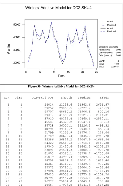
DC2-Sku4 17 1242 2564230
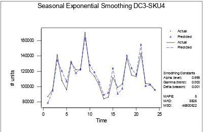
DC3-Sku4 13 3078 16459446
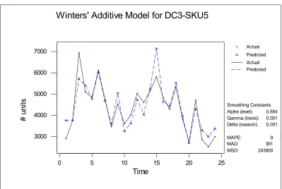
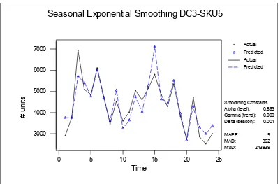
DC3-Sku5 21.4 193.4 60445.9
DC4-Sku4 13 812 1055816
DC5-Sku4 17 1706 4874870
2 ANALYSIS
Simple time series techniques are used to fit the historical sales data. Specifically, deterministic models are fitted and evaluated and then exponential smoothing techniques are used. Finally, regression techniques are used to determine the effect of causals such as housing starts, price and weather on the forecast.
2.1 DETERMINISTIC MODELS
For each of the skus studied, an attempt was first made to fit deterministic models to the time series since these models would be the most simple for the company to implement and they would also shed some light on the nature or structure of the series.
We assume the deterministic model Zt = µt + Xt,
Where Zt is the number of units sold in month t, µt is the mean constant function and Xt is the stochastic or random component.
2.1.1 Seasonal Means Model
The time series plots show blatant seasonal patterns (See Appendix 3). As a result of this observed seasonality, a seasonal means deterministic model is fitted to the series. The seasonal means model (Cryer, 1986) assumes,
µt = µt + 12 for all t
We assume that there are 12 parameters, µ1, µ2, … , µ12 , giving the expected average monthly lumber demand for each of the twelve months. For this model, in the absence of any predictor variables, the seasonal means estimate of βj is just the average of all data at period j for all the seasons.
2.1.2 Cosine Trend Model
µt = β0 + β1 cos (2πt/12) + β2 sin (2πt/12) (5)
An adaptation of the cosine trend model that improved the fit is done. This adapted cosine trend model assumes,
µt = β0t + β1t cos (2πt/12) + β2t sin (2πt/12) (6)
The optimal β1t‘s and β2t‘s were determined using quadratic programming (Winston, 1994) to minimize the sum of the square residuals for each month,
Minimize Σ et2 Subject to:
Ft - Zt - et = 0 for each t
Ft - β0t + β1t cos (2πt/12) + β2t sin (2πt/12) = 0 for each t Ft+12 - β0t + β1t cos (2πt/12) + β2t sin (2πt/12) = 0 for each t
Ft ≥ 0, β0t, β1t, et free
Where Zt is the number of units sold in month t, Ft, a variable, is the forecasted number of units sold in month t and et is the residual.
2.2 SMOOTHING MODELS
If the deterministic models were not appropriate, exponential smoothing models were fitted.
2.2.1 Winters Additive Model
An observation of the time series, shows that the amplitude of the seasonal pattern is not proportional to the average height of the series. Therefore an additive seasonal model is in order (Montgomery et al., 1990). This approach to forecasting a seasonal time series is due to Holt (Holt, 1957) and Winters (Winters, 1960) and is called the Winters additive method. In keeping with the notation already used, we will assume that the time series are adequately represented by the model,
where b1 is the level or permanent component, b2 is the linear trend component and st is the additive seasonal factor. The following iterative procedure, specifically tailored to the available data set of 24 POS monthly observations, is used to fit data at the end of each month, t, and forecast at the end of the sample:
1. The starting (time 0) level and trend are obtained by solving 2 linear equations:
b1(0)
∑
=
24
1 t
t + b2(0)
∑
=
24
1 t
t2 = tZ
t
∑
=
24
1
t (7)
24 b1(0) + 300 b2(0) = Z
t
∑
=
24
1
t (8)
2. The estimate of the permanent component is updated:
b1(t) = [Zt - st (t - 12)] + (1 - α)[b1(t - 1) + b2(t – 1) (9)
where 0< α <1 is the level smoothing constant.
3. The estimate of the trend component is updated.
b2(t) = γ [b1(t) - b1(t - 1)] + (1 - γ)b2(t – 1) (10) where 0<γ<1 is the trend smoothing constant.
4. The estimate of the seasonal factor is updated.
st(t) = δ [Zt - b1(t)] + (1 - δ) st(t-12) (11)
where 0<δ<1 is the seasonal smoothing constant.
2.2.2 Seasonal Exponential Smoothing Model
The Seasonal Exponential Smoothing model is identical to the Winters Additive Method, except that there is no trend component. Therefore, the model equation is,
Zt = b1 + st + Xt
This model only uses the level, α, and seasonal, δ, smoothing constants.
For both Smoothing models, SAS/ETS software4 is used to optimize the smoothing constants by minimizing the sum of squared one-step-ahead prediction errors.
2.2.3 Log Transforms
In some cases, logarithm transformations are done before the smoothing methodology is applied, to obtain approximately constant variance. The logarithmic transform is,
Wt = ln (Zt) (13)
2.3 MODEL EVALUATION
Each model is evaluated based on:
1. Appropriateness: The model is deemed appropriate if its residuals are independent, that is, randomly distributed (Chatfield, 2001). Randomness is determined by observing the autocorrelations. The sample autocorrelation function, rk is defined by,
rk =
∑
∑
=
− +
=
− − −
n
t t
k t n
k t
t
Y Z
Y Z Y Z
1
2 1
] [
] [
] [
for k = 0,1,2,… (14)
Where k is the lag, Zt is the number of units sold in month t and Y is the sample mean. The model is appropriate if the residual autocorrelations do not differ significantly from zero.
2. Fit: The fit statistic used is MAPE (Mean Absolute Percentage Error). This fit statistic is chosen since its unit, percentage, is scale independent (Chatfield, 2001). The MAPE values from the forecasting models recommended in this study, can be compared to the MAPE values achieved in the current moving average forecasting that the company uses. The other fit statistics that Minitab computes, MAD (Mean Absolute Deviation) and MSD (Mean Square Deviation), have values in the units of the data being fit. Since we are comparing weekly data (of the moving averages) to monthly data (of this study), the MAD and MSD are not appropriate.
3. Comparison: The February 2003 data point was used as the out-of-sample validation point. The forecasting model that has the smallest MAPE for this point is deemed the “best” (Chatfield, 2001).
2.4 FORECAST LIMITS
Ryan-Joiner (Ryan, 1976 and Filliben, 1975) normality tests are done on the residuals of the “best” models. Minitab has three tests for normality: Anderson-Darling, Ryan-Joiner and Kolmogorov-Smirnov. The Anderson-Darling and Ryan-Joiner tests have similar power for detecting non-normality. The Kolmogorov-Smirnov test has lesser power because it does not fit the distribution tails well (see D’Augustino, 1986 for discussions of these tests for normality). Therefore, the Ryan-Joiner test was chosen to do the normality analyses.
The common null hypothesis for the Ryan-Joiner tests is,
H0: data follow a normal distribution. If the p-value of the test is less than the significance level, reject H0.
2.5 CAUSAL VARIABLES
3 RESULTS
3.1 TIME SERIES PLOTS
The time series plots for all the DC-Skus show striking seasonal patterns. These plots are shown in Appendix 3. Except for DC1-Sku1, all the time series show demand peaks in April, July and October. As will be shown in Section 3.4, these local maxima are also seen in the housing starts series. DC1-Sku1 has peaks in July, October and December. Also, DC2-Sku1 has its maximum yearly demand in January.
As mentioned in Section 1.2, sku 4 was chosen for DCs in different climatic regions (namely Mid-West, South West, North East and South East) so the climatic effect on the demand could be observed. We find that the seasonal demand changes are more exaggerated in the regions where there are more severe climatic changes. In fact in the Mid-West and North East regions, the demand increases in peak time are as much as 75% and 80% from the previous months. Conversely, in the South West and South East regions, the demand changes are more modest with the highest increases being 47% and 46% respectively.
3.2 BEST FITS
The methodology put forth in the Analysis section was implemented for each of the DC-Sku combinations. The Seasonal Means and Cosine Trend Models, even though they were good fits in most cases, were found to not be appropriate for any of the time series studied because the residuals are not independent; the correlograms for these models had correlation coefficients that differed significantly from zero. A DC-Sku (DC1-Sku1) example of the fit of the Seasonal Means and Cosine Trend models are shown in Figures 1 and 2.
DC1-Sku1Mthly POS/Seasonal Means Series
0 5000 10000 15000 20000 25000
Jan-01 Apr-01 Jul-01 Nov-01 Feb-02 May-02 Sep-02 Dec-02 Mar-03
Month-Year
#unit
s Mthly POS
Series Seasonal Means
Figure 1: Fit of Seasonal Means model to DC1-Sku1 time series
Adapted Cosine Trend / POS Comparison DC1-Sku1
0 5000 10000 15000 20000 25000
Jan-01 Apr-01 Jul-01 Nov-01 Feb-02 May-02 Sep-02 Dec-02 Mar-03 Month-Year
# units
Lingo CosSin POS
Figure 2: Fit of Cosine Trend model to DC1-Sku1 time series
improvement was 3% for DC1-Sku2, which is still a substantial improvement. The average improvement is 11.2%. The proposed improvement in fit accuracy is enough to warrant the extra “trouble” of using the simple exponential smoothing models. In most cases the Seasonal Exponential Smoothing models and Winters Additive models behaved similarly in terms of fit. In the instances when one was better than the other, the MAPEs only differed by 1%. In addition, a smaller MAPE was achieved if the actual POS series was logarithmically transformed (see equation (13)), before the smoothing model was applied. But even in these cases, the improvements were not more than 1%.
DC-SKU MODEL α γ δ
DC1-Sku1 Winters Additive 0.5504 0.0010 0.0010
Seasonal Exponential Smoothing 0.6100 0.0010 Log Seasonal Exponential Smoothing 0.6369 0.0010 DC1-Sku2 Log Winters Additive 0.7445 0.9302 0.9990
Winters Additive 0.8995 0.1872 0.9990
Seasonal Exponential Smoothing 0.9065 0.9990 DC2-Sku3 Seasonal Exponential Smoothing 0.9397 0.9990
Winters Additive 0.9336 0.0018 0.9990
Log Seasonal Exponential Smoothing 0.9314 0.9990 DC2-Sku4 Log Winters Additive 0.9990 0.0010 0.9990
Winters Additive 0.9990 0.0010 0.0010
Seasonal Exponential Smoothing 0.9629 0.9990 DC3-Sku4 Log Winters Additive 0.8600 0.0010 0.0010
Winters Additive 0.8543 0.0010 0.0010
Seasonal Exponential Smoothing 0.9990 0.0010 DC3-Sku5 Seasonal Exponential Smoothing 0.8630 0.0010
Winters Additive 0.8543 0.0010 0.0010
Log Seasonal Exponential Smoothing 0.9990 0.0010 DC4-Sku4 Log Winters Additive 0.1014 0.0010 0.0010
Winters Additive 0.0921 0.0010 0.0010
Seasonal Exponential Smoothing 0.2915 0.0010 DC5-Sku4 Log Seasonal Exponential Smoothing 0.9990 0.0010 Seasonal Exponential Smoothing 0.7829 0.0010
Winters Additive 0.1993 0.9222 0.1065
DC-SKU MODEL MAPE
DC1-Sku1 Winters Additive 10
Seasonal Exponential Smoothing 9 Log Seasonal Exponential Smoothing 10
Moving Average 39
DC1-Sku2 Log Winters Additive 4
Winters Additive 5
Seasonal Exponential Smoothing 5
Moving Average 8
DC2-Sku3 Seasonal Exponential Smoothing 7
Winters Additive 7
Log Seasonal Exponential Smoothing 7
Moving Average 11
DC2-Sku4 Log Winters Additive 5
Winters Additive 5
Seasonal Exponential Smoothing 5
Moving Average 17
DC3-Sku4 Log Winters Additive 5
Winters Additive 5
Seasonal Exponential Smoothing 5
Moving Average 13
DC3-Sku5 Seasonal Exponential Smoothing 9
Winters Additive 9
Log Seasonal Exponential Smoothing 9
Moving Average 21
DC4-Sku4 Log Winters Additive 3
Winters Additive 3
Seasonal Exponential Smoothing 4
Moving Average 13
DC5-Sku4 Log Seasonal Exponential Smoothing 5 Seasonal Exponential Smoothing 6
Winters Additive 6
Moving Average 17
3.3OUT-OF-SAMPLE FORECAST BEHAVIOR
3.3.1 Behavior of Forecast Interval
Appendix 5 shows the correlograms and normality plots for the log-transformed series. All of the residuals from these methods were independent, because the autocorrelation functions were close to zero up to lag 23, and all but one (DC3-Sku4) are normally distributed. Similarly, the residuals from the non-transformed models were all independent and normally distributed (see Appendix 6 for normality plots). We capitalize on the normally distributed residuals of the non-transformed series to obtain a 99% tolerance interval for the forecasts using the standard deviation of the residuals and multiplying that value by the z-score 2.58. Table 5 shows that the Actual lumber demand for February 2003 fell within this 99% tolerance interval for all the DC-Skus.
3.3.2 Accuracy Comparison of Forecast
The February 2003 forecasts produced by the non-transformed Winters Additive and Seasonal Exponential Smoothing models are compared to the actual lumber demand observed for that month. The non-transformed series are used because these are simpler to actually implement, and provided similar, if not better fits than the log transformed models (see Table 5). The Absolute Percentage Error (APE) is also compared to the MAPE obtained from the 7-week Moving Average (MA) model discussed in Section 1.4. The APE equation is identical to the MAPE equation (1), when n=1.
The Moving Average February 2003 forecast is compared to the forecast obtained using the two smoothing models in Table 6. There was a drastic decrease in demand for DC1-Sku1 in February 2003, the demand was 1598 units compared to February 2001 and February 2002, where the demand was 3135 units and 5395 units respectively. The Smoothing models, therefore, do not perform well in forecasting the DC1-Sku1 February 2003 demand. Because the average is obtained every week, the moving average model performs better, but still very badly in forecasting the DC1-Sku1 February 2003 demand. For the other seven DC-Skus, the smoothing models performed better for three (3) and the Moving Average model performed better for three (3), while for DC5-Sku4, the Winters Additive method performed the best and the Moving Average model performed better than the Seasonal Exponential Smoothing model. Therefore, no conclusive statement can be made about which model performs better in this out-of-sample analysis. We can say, however, that the Moving Average model responds more quickly to drastic deviations from the historical trend.
3.4 CAUSAL VARIABLES RESULTS
The time series of the causal variables, suggested by the DC Inventory Managers and trade associations such as WWPA, are studied. The causal factors observed are non-seasonally adjusted new housing starts in the DC region5, monthly average temperature in the DC region6 and price7. Step-wise regressions were performed on causals because the causal factors may be interdependent; step-wise regression first removes these interdependencies. The regression was done for the DC-Skus in the North East, Mid-West and South West.
5 The housing starts data was obtained from the US Census Bureau Website
http://www.census.gov
6 The monthly average temperature was obtained from the National Weather Services Website
http://www.weather.gov
7 Random Lengths price data was used
99% TOLERANCE INTERVAL
DC-SKU MODEL FORECAST ACTUAL ERROR UPPER LOWER APE MAPEMA
Winters
Additive 3583 1598 -1985 5907 1259 124 75
DC1-Sku1
Seasonal Exponential
Smoothing 3518 1598 -1920 5830 1206 120 75
Winters
Additive 111594 105082 -6512 133115 90073 6 22
DC1-Sku2
Seasonal Exponential
Smoothing 121198 105082 -16116 143479 98917 15 22
Winters
Additive 537972 560733 22761 643709 432235 4 6
DC2-Sku3
Seasonal Exponential
Smoothing 538818 560733 21915 644382 433254 4 6
Winters
Additive 16966 20368 3402 21581 12351 17 5
DC2-Sku4
Seasonal Exponential
Smoothing 17024 20368 3344 21740 12308 16 5
Winters
Additive 82514 78826 -3688 100191 64837 5 21
DC3-Sku4
Seasonal Exponential
Smoothing 82542 78826 -3716 99914 65170 5 21
Winters
Additive 2104 3192 1088 3395 813 34 17
DC3-Sku5
Seasonal Exponential
Smoothing 2102 3192 1090 3393 811 34 17
Winters
Additive 20809 22872 2063 24080 17538 9 5
DC4-Sku4
Seasonal Exponential
Smoothing 20789 22872 2083 24300 17278 9 5
Winters
Additive 23676 23031 -645 32052 15300 3 17
DC5-Sku4
Seasonal Exponential
3.4.1 Housing Starts Series
The plots of the housing starts time series in each of the DC regions observed are shown in Figures 3 through 5. The plots show local maxima in the Spring, Summer and Fall, however, the maxima do not always take place in April, July and October, as is the case for the Point-of-Sale local maxima. For example, for DC2, the housing starts Spring peaks occur in April 2001 and March 2002. Similarly, the Summer peaks occur in July 2001 and June 2002. Since the local maxima did not occur at the same time, none of the correlations between the POS series and the housing starts series exceeded 0.71 and for four of the six DC-Skus observed, the correlation was less than 0.4.
3.4.2 Average Monthly Temperature Series
The monthly average temperature varies as expected, with highs in the summer months and lows in the winter. These series did not show the lumpiness of the local maxima in the Spring, Summer and Fall as observed in the Point-of-Sale and Housing Starts Time Series. The monthly average temperature series are shown in Appendix 7. Because there was no lumpiness in the monthly average temperature series, the correlations of this series with the POS series did not exceed 0.78 and in three of the six cases, it was less than 0.4.
3.4.3 Price Series
There was very little variation in the random lengths price data during 2001 and 2002. In some cases, the price remained exactly the same throughout the entire period. In other cases, only one month recorded any change and even in these cases, the change was not substantial. Therefore, there was no correlation between the price series and the POS series over the two-year observation period.
3.4.4 Step-wise regression
regression study is shown in Appendix 8. One interpretation of R2 is that it is the square of the sample correlation coefficient between the observed series and the assumed trend (Cryer, 1986, page 40). Therefore, a R2 value of 65% means that, 65% of the variation in the monthly POS
DC1 Housing Starts Series
0 2 4 6 8 10 12 14 16 18 20
Jan-01 Apr-01 Jul-01 Nov-01 Feb-02 May-02 Sep-02 Dec-02 Mar-03
Month-Year
#unit
s in t
housands
Figure 3: Housing Starts Time Series for DC18
DC2 Housing Starts Series
0 5 10 15 20 25 30 35 40
Jan-01 Apr-01 Jul-01 Nov-01 Feb-02 May-02 Sep-02 Dec-02 Mar-03
Month-Year
# units in thousands
Figure 4: Housing Starts Time Series for DC29
DC3 Housing Starts Series
0 5 10 15 20 25 30 35 40 45
Jan-01 Apr-01 Jul-01 Nov-01 Feb-02 May-02 Sep-02 Dec-02 Mar-03
Month- Year
# units in thousands
Figure 5: Housing Starts Time Series for DC310
time series is explained by the proposed regression model. The R2 values obtained suggest that none of the proposed causals should be used as predictor variables.
9The DC2 Housing Starts Series has peaks in June, August and October of 2001 and May, September and
November of 2002.
10
4
CONCLUSION AND RECOMMENDATIONS
The Smoothing models proposed in this paper, meet the criteria set forth by the company (see section 1.1); The Seasonal Exponential Smoothing and Winters Additive models are simple, easy to implement in the existing Minitab software available at the company, and since the residuals obtained from these models were normally distributed, the 99% tolerance interval to maintain the fill rate could be found. The out-of-sample forecasts for the smoothing models all fell within the 99% tolerance interval proposed.
The monthly forecasting would serve to facilitate decision making in light of the long lead times and does well to predict season changes. The smoothing models have better “ramp-up” and “ramp-down” properties, when the skus are coming into season and going out of season respectively, as observed in the time series plots in Appendix 4. The smoothing models also have better MAPE fit statistics than the Moving Average models as discussed in section 3.
No conclusive statement can be made, from the current out-of-sample analyses done, about whether any of the models (smoothing or Moving Average) behave better, except that the smoothing models would allow the DC inventory Manager to “look further ahead” more accurately. Both the Seasonal Exponential Smoothing and Winters Additive models have similar out-of-sample performance. They both perform badly when there is a drastic shift away from the historical trend as is the case with DC1-Sku1 February 2003. The Moving Average model captures the drastic shifts more quickly (although it still behaved badly in the DC1-Sku1 February 2003 case) because it is reviewed weekly. The author, therefore, recommends that the monthly smoothing models be used to plan ahead for seasonality changes, and the actual demand be reviewed weekly to determine whether the historical trend is being followed. For example if the actual demand for the first week of a particular month is only 10% of the forecasted demand for that month, then one can predict that that month is going to have unusually low demand and adjust shipment decisions accordingly.
5 FUTURE
WORK
Further observation of the out-of-sample behavior of the forecasting smoothing models proposed is required. As more demand data becomes available, the forecasting accuracy of the model will be continuously evaluated and updated.
The methodology would be implemented at the company (theoretically) for all the skus at the “problem” DCs where there are space constraints to determine the realizable average inventory turns possible.
The company plans to develop a tool that considers the on-hand lumber inventory, the expected inbound inventory and the forecasted demand to predict overages and shortages. The process will then be piloted (physically implemented) at one of the DCs. If the pilot is successful, the process would then be implemented at other “problem” DCs.
6 REFERENCES
Armstrong, J. S. (2001). Principles of Forecasting, Kluwer Academic Press.
Armstrong, J.S.(1984). Forecasting by Extrapolation : Conclusions from twenty-Five Year Research.” Interfaces 14, (p. 52-56)
Chatfield, Chris (2001). Time-Series Forecasting, Chapman and Hall/CRC.
Chatfield, Chris (1975). Analysis of Time Series Theory and Practice, Chapman and Hall. Cryer, Jonathan (986). Time Series Analysis, Duxbury Press.
D'Augostino, R. B. and M.A. Stevens, Eds. (1986). Goodness-of-Fit Techniques, Marcel Dekker. Dorn, H. F. (1950), “Pitfalls in population forecasts and projections,” Journal of the American
Statistical Association, 45, (p. 311-334).
Filliben, J. J. (1975). "The Probability Plot Correlation Coefficient Test for Normality,"
Technometrics, Vol 17, (p.111).
Holt, C. C. (1957) “Forecasting Seasonal and Trends by Exponentially Weighted Moving Averages.” Office of naval research memorandum (No. 52).
McCullagh, P. and J.A. Nelder (1992). Generalized Linear Models, Chapman & Hall.
Montgomery, Douglas C., L.A. Johnson and J. S. Gardiner (1990). Forecasting and Time Series
Analysis, McGraw Hill.
Nahmias, S. (2001). Production and Operations Analysis, McGraw Hill.
Rich, S. U. (1970). Marketing of Forest Products: Text and Cases, McGraw Hill.
Ryan, T. A. Jr. and B.L. Joiner (1976). "Normal Probability Plots and Tests for Normality," Technical Report, Statistics Department, The Pennsylvania State University.
Shapiro S.S. and R.S. Francia (1972). "An Approximate Analysis of Variance Test for Normality," Journal of the American Statistical Association, Vol 67, 215.
Stephens, M. A. (1974). EDF Statistics for Goodness of Fit and Some Comparisons, Journal of
the American Statistical Association, Vol. 69, 730-737.
Winston, Wayne L. (1994). Operations Research: Applications an Algorithms, Duxbury Press. Winters, P. R. (1960). “Forecasting Sales by Exponentially Weighted Moving Averages.”
7 APPENDICES
APPENDIX 1
POS-Transfer Comparisons for skus that showed little correlation
DC1-Sku2 POS Transfer Comparison
0 50000 100000 150000 200000 250000
Jul-01 Nov-01 Feb-02 May-02 Sep-02 Dec-02 Mar-03
Month-Year
# units
POS Transfers
DC4-Sku4 POS Transfer Comparison
0 5000 10000 15000 20000 25000 30000 35000 40000
Jul-01 Nov-01 Feb-02 May-02 Sep-02 Dec-02 Mar-03
Month-Year
# units
POS Transfer
APPENDIX 2
Time Series Plots of AS-IS Moving Average Forecasting models11
Actual Predicted Actual Predicted
100 50
0 8500
7500
6500
5500
4500
3500
2500
1500
500
DC
1
-S
ku
1
W
kl
Time
MSD: MAD: MAPE: Length: Moving Average
1190011 781 39 7
DC1-SKU1 Moving Average (7 Weeks)
Figure 8: 7-Week Moving Average Time Series for DC1-Sku1
Actual Predicted Actual Predicted
0 50 100
25000 35000 45000
DC
1
-S
ku
2
W
kl
Time
Moving Average Length:
MAPE: MAD: MSD:
7
8 2731 14587294
DC1-SKU2 Moving Average (7 Weeks)
Actual Predicted Actual Predicted
100 50
0 180000
130000
80000
DC
2
-S
ku
3
W
kl
Time
MSD: MAD: MAPE: Length: Moving Average
2.26E+08 12268 11 7
DC2-SKU3 Moving Average (7 Weeks)
Figure 10: 7-Week Moving Average Time Series for DC2-Sku3
Actual Predicted Actual Predicted
100 50
0 12500
10000
7500
5000
DC
2
-S
ku
4
W
kl
Time
MSD: MAD: MAPE: Length: Moving Average
2564230 1242 17 7
DC2-SKU4 Moving Average (7 Weeks)
Actual Predicted Actual Predicted
100 50
0 35000
25000
15000
DC
3
-S
ku
4
W
kl
Time
MSD: MAD: MAPE: Length: Moving Average
16459446 3078 13 7
DC3-SKU4 Moving Average (7 Weeks)
Figure 12: 7-Week Moving Average Time Series for DC3-Sku4
Actual Predicted Actual Predicted
100 50
0 1500
1000
500
DC
3
-S
ku
5
W
kl
Time
MSD: MAD: MAPE: Length: Moving Average
60445.9 193.4 21.4 7
DC3-SKU5 Moving Average (7 Weeks)
Actual Predicted Actual Predicted
100 50
0 10500
9500
8500
7500
6500
5500
4500
3500
DC
4
-S
ku
4
W
kl
Time
MSD: MAD: MAPE: Length: Moving Average
1055816 812 13 7
DC4-SKU4 Moving Average (7 Weeks)
Figure 14: 7-Week Moving Average Time Series for DC4-Sku4
Actual Predicted Actual Predicted
100 50
0 15000
10000
5000
DC
5
-S
ku
4
W
kl
Time
MSD: MAD: MAPE: Length: Moving Average
4874870 1706 17 7
DC5-SKU4 Moving Average (7 Weeks)
APPENDIX 3
Monthly Point-of-Sale Time Series Plots for the DC-Skus
DC1-Sku1 Monthly POS Series
0 5000 10000 15000 20000 25000
Jan-01
Feb-01
Apr-01
Jun-01
Jul-01 Sep-01
Nov-01
Dec-01
Feb-02
Apr-02
May-02
Jul-02 Sep-02
Oct-02
Dec-02
Jan-03
Mar-03
May-03
Month-Year
#units
Figure 16: Monthly POS time series for DC1-Sku1
DC1-Sku2 POS Time Series
0 50000 100000 150000 200000 250000
Jan-01 Apr-01 Jul-01 Nov-01 Feb-02 May-02 Sep-02 Dec-02 Mar-03 Jun-03
Month-Year
# unit
s
DC2-SKU3 POS Time Series
0 100000 200000 300000 400000 500000 600000 700000 800000
Jan-01 Apr-01 Jul-01 Nov-01 Feb-02 May-02 Sep-02 Dec-02 Mar-03 Month-Year
# units
Figure 18: Monthly POS time series for DC2-Sku3
DC2-SKU4 POS Time Series
0 10000 20000 30000 40000 50000 60000
Jan-01 Apr-01 Jul-01 Nov-01 Feb-02 May-02 Sep-02 Dec-02 Mar-03 Jun-03 Month-Year
# units
DC3-Sku4 Mthly POS Series
0 20000 40000 60000 80000 100000 120000 140000 160000 180000
Jan-01 Apr-01 Jul-01 Nov-01 Feb-02 May-02 Sep-02 Dec-02 Mar-03 Jun-03
Month-Year
# unit
s sold
Figure 20: Monthly POS time series for DC3-Sku4
DC3-Sku5 Mthly POS Series
0 1000 2000 3000 4000 5000 6000 7000 8000
Jan-01 Apr-01 Jul-01 Nov-01 Feb-02 May-02 Sep-02 Dec-02 Mar-03 Jun-03
Month-Year
# unit
s
DC4-Sku4 Mthy POS Series
0 5000 10000 15000 20000 25000 30000 35000 40000 45000
Jan-01 Apr-01 Jul-01 Nov-01 Feb-02 May-02 Sep-02 Dec-02 Mar-03
Month-Year
# unit
s sold
Figure 22: Monthly POS time series for DC4-Sku4
DC5-Sku4 Mthly POS Series
0 10000 20000 30000 40000 50000 60000 70000 80000
Jan-01 Apr-01 Jul-01 Nov-01 Feb-02 May-02 Sep-02 Dec-02 Mar-03
Month-Year
# unit
s
APPENDIX 4
Time Series Plots for the Winters Additive and Seasonal Exponential Smoothing Models in Table 412
DC1-SKU1
Actual Predicted Actual Predicted
25 20
15 10
5 0
22000
12000
2000
#
uni
ts
Time
MSD: MAD: MAPE: Delta (season): Gamma (trend): Alpha (level): Smoothing Constants
780377 768 10 0.001 0.001 0.550
Winters' Additive Model for DC1-SKU1
Figure 24: Winters Additive Model for DC1-SKU1
Row Time DC1-SKU1 POS Smooth Predict Error
Actual Predicted Actual Predicted
25 20
15 10
5 0
22000
12000
2000
#
uni
ts
Time
MSD: MAD: MAPE: Delta (season): Gamma (trend): Alpha (level): Smoothing Constants
771799 746 9 0.001 0.000 0.610
Seasonal Exponential Smoothing DC1-SKU1
Figure 25: Seasonal Exponential Smoothing Model for DC1-SKU1
Row Time DC1-SKU1 POS Smooth Predict Error
DC1-SKU2
Actual Predicted Actual Predicted
25 20
15 10
5 0
220000
170000
120000
#
uni
ts
Time
MSD: MAD: MAPE: Delta (season): Gamma (trend): Alpha (level): Smoothing Constants
71517257 7302 5 0.999 0.187 0.900
Winters' Additive Model for DC1-SKU2
Figure 26: Winters Additive Model for DC1-SKU2
Row Time DC1-SKU2 POS Smooth Predict Error
Actual Predicted Actual Predicted
25 20
15 10
5 0
220000
170000
120000
# u
its
Time
MSD: MAD: MAPE: Delta (season): Gamma (trend): Alpha (level): Smoothing Constants
97307658 8373 5 0.999 0.000 0.906
Seasonal Exponential Smoothing DC1-SKU2
Figure 27: Seasonal Exponential Smoothing Model for DC1-SKU2
Row Time DC1-SKU2 POS Smooth Predict Error
DC2-SKU3
Actual Predicted Actual Predicted
25 20
15 10
5 0
700000
600000
500000
400000
300000
#
uni
ts
Time
MSD: MAD: MAPE: Delta (season): Gamma (trend): Alpha (level): Smoothing Constants
1.98E+09 33746 7 0.999 0.002 0.934
Winters' Additive Model for DC2-SKU3
Figure 28: Winters Additive Model for DC2-SKU3
Row Time DC2-SKU3 POS Smooth Predict Error
Actual Predicted Actual Predicted
0 5 10 15 20 25
300000 400000 500000 600000 700000
#
uni
ts
Time
Smoothing Constants Alpha (level): Gamma (trend): Delta (season):
MAPE: MAD: MSD:
0.940 0.000 0.999
7 33781 1.98E+09
Seasonal Exponential Smoothing DC2-SKU3
Figure 29: Seasonal Exponential Smoothing Model for DC2-SKU3
Row Time DC2-SKU3 POS Smooth Predict Error
DC2-SKU4
Actual Predicted Actual Predicted
25 20
15 10
5 0
50000
40000
30000
20000
#
uni
ts
Time
MSD: MAD: MAPE: Delta (season): Gamma (trend): Alpha (level): Smoothing Constants
3239717 1503 5 0.001 0.001 0.999
Winters' Additive Model for DC2-SKU4
Figure 30: Winters Additive Model for DC2-SKU4
Row Time DC2-SKU4 POS Smooth Predict Error
Actual Predicted Actual Predicted
25 20
15 10
5 0
50000
40000
30000
20000
#
uni
ts
Time
MSD: MAD: MAPE: Delta (season): Gamma (trend): Alpha (level): Smoothing Constants
3390202 1539 5 0.999 0.000 0.963
Seasonal Exponential Smoothing DC2-SKU4
Figure 31: Seasonal Exponential Smoothing Model for DC2-SKU4
Row Time DC2-SKU4 POS Smooth Predict Error
DC3-SKU4
Actual Predicted Actual Predicted
0 5 10 15 20 25
80000 100000 120000 140000 160000
#
uni
ts
Time
Smoothing Constants Alpha (level): Gamma (trend): Delta (season):
MAPE: MAD: MSD:
0.854 0.001 0.001
5 6001 49452144
Winters' Additive Model for DC3-SKU4
Figure 32: Winters Additive Model for DC3-SKU4
Row Time DC3-SKU4 POS Smooth Predict Error
Actual Predicted Actual Predicted
0 5 10 15 20 25
80000 100000 120000 140000 160000
#
uni
ts
Time
Smoothing Constants Alpha (level): Gamma (trend): Delta (season):
MAPE: MAD: MSD:
0.999 0.000 0.001
5 5826 46800522
Seasonal Exponential Smoothing DC3-SKU4
Figure 33: Seasonal Exponential Smoothing Model for DC3-SKU4
Row Time DC3-SKU4 POS Smooth Predict Error
DC3-SKU5
Actual Predicted Actual Predicted
0 5 10 15 20 25
3000 4000 5000 6000 7000
#
uni
ts
Time
Smoothing Constants Alpha (level): Gamma (trend): Delta (season):
MAPE: MAD: MSD:
0.854 0.001 0.001
9 361 243800
Winters' Additive Model for DC3-SKU5
Figure 34: Winters Additive Model for DC3-SKU5
Row Time DC3-SKU5 POS Smooth Predict Error
Actual Predicted Actual Predicted
0 5 10 15 20 25
3000 4000 5000 6000 7000
#
uni
ts
Time
Smoothing Constants Alpha (level): Gamma (trend): Delta (season):
MAPE: MAD: MSD:
0.863 0.000 0.001
9 362 243839
Seasonal Exponential Smoothing DC3-SKU5
Figure 35: Seasonal Exponential Smoothing Model for DC3-SKU5
Row Time DC3-SKU5 POS Smooth Predict Error
DC4-SKU4
Actual Predicted Actual Predicted
0 5 10 15 20 25
22000 32000 42000
#
uni
ts
Time
Smoothing Constants Alpha (level): Gamma (trend): Delta (season):
MAPE: MAD: MSD:
0.092 0.001 0.001
3 1008 1579144
Winters' Additive Model for DC4-SKU4
Figure 36: Winters Additive Model for DC4-SKU4
Row Time DC4-SKU4 POS Smooth Predict Error
Actual Predicted Actual Predicted
0 5 10 15 20 25
22000 32000 42000
#
uni
ts
Time
Smoothing Constants Alpha (level): Gamma (trend): Delta (season):
MAPE: MAD: MSD:
0.292 0.000 0.001
4 1027 1783330
Seasonal Exponential Smoothing DC4-SKU4
Figure 37: Seasonal Exponential Smoothing Model for DC4-SKU4
Row Time DC4-SKU4 POS Smooth Predict Error
DC5-SKU4
Actual Predicted Actual Predicted
0 5 10 15 20 25
18000 28000 38000 48000 58000 68000 78000
#
uni
ts
Time
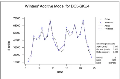
Smoothing Constants Alpha (level): Gamma (trend): Delta (season):
MAPE: MAD: MSD:
0.200 0.922 0.106
6 2655 10697385
Winters' Additive Model for DC5-SKU4
Figure 38: Winters Additive Model for DC5-SKU4
Row Time DC5-SKU4 POS Smooth Predict Error
Actual Predicted Actual Predicted
0 5 10 15 20 25
20000 30000 40000 50000 60000 70000 80000
#
uni
ts
Time
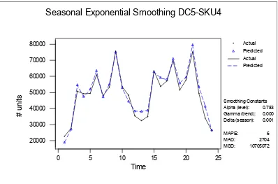
Smoothing Constants Alpha (level): Gamma (trend): Delta (season):
MAPE: MAD: MSD:
0.783 0.000 0.001
6 2704 10705072
Seasonal Exponential Smoothing DC5-SKU4
Figure 39: Seasonal Exponential Smoothing Model for DC5-SKU4
Row Time DC5-SKU4 POS Smooth Predict Error
APPENDIX 5
Correlograms and Normality Plots for the Log-Transformed Smoothing Models in Table 5
22 12 2 1.0 0.8 0.6 0.4 0.2 0.0 -0.2 -0.4 -0.6 -0.8 -1.0 Au to co rr e la tio n LBQ T Corr Lag LBQ T Corr Lag LBQ T Corr Lag LBQ T Corr Lag 29.84 29.83 29.83 29.73 29.62 29.50 29.49 29.47 29.32 28.36 25.73 22.77 12.86 11.37 10.71 10.66 10.50 10.50 10.44 10.16 10.14 9.97 6.40 -0.01 -0.00 -0.07 0.08 0.09 0.04 0.04 -0.14 -0.37 -0.66 -0.75 -1.57 -0.64 -0.45 0.13 -0.23 -0.02 -0.15 -0.34 0.09 0.28 1.43 2.38 -0.00 -0.00 -0.02 0.03 0.03 0.01 0.01 -0.04 -0.12 -0.21 -0.23 -0.44 -0.18 -0.12 0.03 -0.06 -0.01 -0.04 -0.09 0.03 0.08 0.35 0.49 23 22 21 20 19 18 17 16 15 14 13 12 11 10 9 8 7 6 5 4 3 2 1
ACF: DC1-Sku1 Log Seasonal Exponential Smoothing Residuals
Figure 40: Correlogram of DC1-Sku1 Log Seasonal Exponential Smoothing Residuals
StDev: 1304.51 N: 24
W-test for Normality R: 0.9706 P-Value (approx): > 0.1000
-3000 -2000 -1000 0 1000
.001 .01 .05 .20 .50 .80 .95 .99 .999 P rob ab ilit y Smoothing
Normal Probability Plot: DC1-Sku1 Log Seasonal Exponential
22 12 2 1.0 0.8 0.6 0.4 0.2 0.0 -0.2 -0.4 -0.6 -0.8 -1.0 Au to co rr e la tio n LBQ T Corr Lag LBQ T Corr Lag LBQ T Corr Lag LBQ T Corr Lag 21.22 21.21 20.85 20.84 20.52 20.24 20.22 20.11 20.05 19.96 19.76 19.76 12.63 12.55 9.29 9.23 9.17 6.38 6.38 4.29 3.98 3.75 0.10 -0.02 -0.12 -0.03 0.15 -0.16 0.04 0.12 0.09 0.13 0.19 -0.03 -1.38 -0.15 1.05 0.15 -0.15 1.13 -0.01 -1.08 -0.43 -0.39 -1.75 0.30 -0.01 -0.03 -0.01 0.04 -0.05 0.01 0.04 0.03 0.04 0.06 -0.01 -0.37 -0.04 0.27 0.04 -0.04 0.28 -0.00 -0.25 -0.10 -0.09 -0.36 0.06 23 22 21 20 19 18 17 16 15 14 13 12 11 10 9 8 7 6 5 4 3 2 1
ACF: DC1-Sku2 Log Winters' Additive Residuals
Figure 42: Correlogram of DC1-Sku2 Log Winters Additive Residuals
P-Value (approx): > 0.1000 R: 0.9867 W-test for Normality
N: 24 StDev: 8932.02 10000 0 -10000 -20000 .999 .99 .95 .80 .50 .20 .05 .01 .001 P rob ab ilit y
Normal Probability Plot: DC1-Sku2 Log Winters' Additive
22 12 2 1.0 0.8 0.6 0.4 0.2 0.0 -0.2 -0.4 -0.6 -0.8 -1.0 Au to co rr e la tio n LBQ T Corr Lag LBQ T Corr Lag LBQ T Corr Lag LBQ T Corr Lag 35.77 35.45 31.29 27.21 26.96 26.75 25.76 25.57 24.92 24.92 24.91 24.65 12.96 12.87 9.91 5.91 5.82 4.45 4.21 3.08 2.18 1.30 0.61 -0.07 -0.38 -0.46 -0.13 0.14 -0.32 -0.15 -0.30 -0.01 0.04 -0.23 -1.78 -0.16 1.01 1.30 -0.20 -0.83 0.36 0.83 0.77 -0.81 -0.75 0.73 -0.02 -0.12 -0.14 -0.04 0.04 -0.10 -0.05 -0.09 -0.00 0.01 -0.07 -0.47 -0.04 0.26 0.31 -0.05 -0.19 0.08 0.19 0.17 -0.17 -0.16 0.15 23 22 21 20 19 18 17 16 15 14 13 12 11 10 9 8 7 6 5 4 3 2 1
ACF: DC2-Sku3 Log Seasonal Exponential Smoothing Residuals
Figure 44: Correlogram of DC2-Sku3 Log Seasonal Exponential Smoothing Residuals
StDev: 45279.8 N: 24
W-test for Normality R: 0.9721 P-Value (approx): > 0.1000
-100000 -50000 0 50000
.001 .01 .05 .20 .50 .80 .95 .99 .999 P rob ab ilit y Smoothing
Normal Probability Plot: DC2-Sku3 Log Seasonal Exponential
22 12 2 1.0 0.8 0.6 0.4 0.2 0.0 -0.2 -0.4 -0.6 -0.8 -1.0 Au to co rr e la tio n LBQ T Corr Lag LBQ T Corr Lag LBQ T Corr Lag LBQ T Corr Lag 46.54 45.59 45.45 39.04 38.60 38.28 37.43 36.19 34.70 33.51 33.51 33.46 21.17 20.43 20.17 12.06 11.40 9.71 9.41 6.58 5.02 0.48 0.38 0.11 0.06 -0.51 -0.16 -0.15 0.27 0.35 0.41 0.39 -0.01 -0.09 -1.61 -0.41 -0.26 1.63 0.49 0.83 -0.36 -1.20 -0.95 -1.88 0.28 0.58 0.04 0.02 -0.18 -0.05 -0.05 0.09 0.12 0.14 0.13 -0.00 -0.03 -0.49 -0.12 -0.08 0.44 0.13 0.22 -0.09 -0.29 -0.22 -0.39 0.06 0.12 23 22 21 20 19 18 17 16 15 14 13 12 11 10 9 8 7 6 5 4 3 2 1
ACF: DC2-Sku4 Log Winters' Additive Residuals
22 12 2 1.0 0.8 0.6 0.4 0.2 0.0 -0.2 -0.4 -0.6 -0.8 -1.0 A ut o co rr el at ion LBQ T Corr Lag LBQ T Corr Lag LBQ T Corr Lag LBQ T Corr Lag 43.41 43.18 42.69 42.27 41.29 39.63 34.42 34.41 32.40 28.63 28.03 27.08 15.29 14.58 14.37 14.09 12.83 11.26 9.61 9.17 6.86 2.82 1.64 0.06 0.12 0.13 -0.23 -0.34 -0.68 0.03 0.49 0.73 0.31 -0.41 -1.67 -0.43 0.25 0.29 0.65 0.77 0.83 -0.45 -1.10 -1.64 -0.95 1.20 0.02 0.04 0.04 -0.08 -0.12 -0.22 0.01 0.16 0.23 0.10 -0.13 -0.48 -0.12 0.07 0.08 0.18 0.21 0.22 -0.12 -0.27 -0.37 -0.20 0.25 23 22 21 20 19 18 17 16 15 14 13 12 11 10 9 8 7 6 5 4 3 2 1
ACF: DC3-Sku4 Log Winters' Additive Residuals
Figure 47: Correlogram of DC3-Sku4 Log Winters Additive Residuals
StDev: 5911.10 N: 24
W-test for Normality R: 0.9821 P-Value (approx): > 0.1000
-10000 -5000 0 5000
.001 .01 .05 .20 .50 .80 .95 .99 .999 P rob ab ilit y
Normal Probability Plot: DC3-Sku4 Log Winters' Additive
22 12 2 1.0 0.8 0.6 0.4 0.2 0.0 -0.2 -0.4 -0.6 -0.8 -1.0 A ut o co rr el at ion LBQ T Corr Lag LBQ T Corr Lag LBQ T Corr Lag LBQ T Corr Lag 24.77 24.75 24.64 24.63 22.69 22.48 20.47 20.33 20.31 20.23 19.06 18.92 6.25 6.24 5.84 5.81 3.31 3.29 2.62 2.53 1.98 1.91 0.11 0.02 0.07 0.02 -0.39 -0.15 0.49 -0.14 -0.05 -0.13 0.49 0.18 -2.07 0.06 0.40 -0.10 1.12 0.12 -0.63 0.23 -0.61 0.23 -1.23 -0.31 0.01 0.02 0.01 -0.11 -0.04 0.14 -0.04 -0.01 -0.04 0.14 0.05 -0.49 0.02 0.10 -0.02 0.25 0.03 -0.14 0.05 -0.13 0.05 -0.25 -0.06 23 22 21 20 19 18 17 16 15 14 13 12 11 10 9 8 7 6 5 4 3 2 1
ACF: DC3-Sku5 Log Seasonal Exponential Smoothing Residuals
Figure 49: Correlogram of DC3-Sku5 Log Seasonal Exponential Smoothing Residuals
P-Value (approx): 0.0483 R: 0.9561 W-test for Normality
N: 24 StDev: 582.166 1000 0 -1000 .999 .99 .95 .80 .50 .20 .05 .01 .001 P rob ab ilit y
Normal Probability Plot: DC3-Sku5 Log Seasonal Exponential Smoothing
22 12 2 1.0 0.8 0.6 0.4 0.2 0.0 -0.2 -0.4 -0.6 -0.8 -1.0 A ut o co rr el at ion LBQ T Corr Lag LBQ T Corr Lag LBQ T Corr Lag LBQ T Corr Lag 53.27 51.89 51.47 44.12 43.18 42.04 39.67 39.40 38.60 37.72 35.53 35.52 22.83 22.41 21.80 12.90 12.84 10.55 9.72 8.33 7.76 3.29 0.04 0.13 0.10 -0.53 -0.22 0.27 0.43 -0.16 -0.29 0.33 0.55 0.04 -1.59 -0.30 0.38 1.68 0.15 -0.94 -0.59 0.80 0.53 -1.71 -1.66 0.18 0.05 0.04 -0.19 -0.08 0.10 0.15 -0.06 -0.10 0.11 0.19 0.01 -0.49 -0.09 0.12 0.46 0.04 -0.25 -0.15 0.21 0.13 -0.39 -0.34 0.04 23 22 21 20 19 18 17 16 15 14 13 12 11 10 9 8 7 6 5 4 3 2 1
ACF: DC4-Sku4 Log Winters' Additive Residuals
Figure 51: Correlogram of DC4-Sku4 Log Winters Additive Residuals
StDev: 1214.47 N: 24
W-test for Normality R: 0.9734 P-Value (approx): > 0.1000
-3000 -2000 -1000 0 1000 2000 3000
.001 .01 .05 .20 .50 .80 .95 .99 .999 P rob ab ilit y
Normal Probability Plot: DC4-Sku4 Log Winters' Additive
22 12 2 1.0 0.8 0.6 0.4 0.2 0.0 -0.2 -0.4 -0.6 -0.8 -1.0 A ut o co rr el at ion LBQ T Corr Lag LBQ T Corr Lag LBQ T Corr Lag LBQ T Corr Lag 32.07 31.58 30.66 28.25 27.12 22.93 22.76 21.77 21.76 21.39 19.41 19.40 8.64 7.58 7.22 6.62 6.47 3.95 3.90 3.90 3.90 3.79 0.84 0.09 -0.18 -0.36 -0.29 -0.63 -0.14 -0.37 -0.03 -0.25 -0.63 -0.06 -1.81 -0.60 -0.36 0.49 0.25 1.14 0.15 -0.06 -0.03 0.25 1.54 0.86 0.03 -0.05 -0.11 -0.09 -0.18 -0.04 -0.11 -0.01 -0.07 -0.18 -0.02 -0.45 -0.15 -0.09 0.12 0.06 0.26 0.04 -0.01 -0.01 0.06 0.32 0.18 23 22 21 20 19 18 17 16 15 14 13 12 11 10 9 8 7 6 5 4 3 2 1
ACF: DC5-Sku4 Log Seasonal Exponential Smoothing Residuals
Figure 53: Correlogram of DC5-Sku4 Log Seasonal Exponential Smoothing Residuals
P-Value (approx): > 0.1000 R: 0.9847 W-test for Normality
N: 24 StDev: 2597.15 5000 0 -5000 .999 .99 .95 .80 .50 .20 .05 .01 .001 P rob ab ilit y
Normal Probability Plot: DC5-Sku4 Log Seasonal Exponential Smoothing
APPENDIX 6
Normality Plots for the Non-Transformed Smoothing Models in Table 513
StDev: 902.381 N: 24
W-test for Normality R: 0.9907 P-Value (approx): > 0.1000
-1000 0 1000
.001 .01 .05 .20 .50 .80 .95 .99 .999
P
rob
ab
ilit
y
Normality Probability Plot: DC1-Sku1 Winters' Additive
Figure 55: Normal Plot of DC1-Sku1 Winters Additive Residuals
StDev: 897.386 N: 24
W-test for Normality R: 0.9948 P-Value (approx): > 0.1000
-1000 0 1000
.001 .01 .05 .20 .50 .80 .95 .99 .999
P
rob
ab
ilit
y
Normality Probability Plot: DC1-Sku1 Seasonal Exponential Smoothing
Figure 56: Normal Plot of DC1-Sku1 Seasonal Exponential Smoothing Residuals
StDev: 8355.03 N: 24
W-test for Normality R: 0.9805 P-Value (approx): > 0.1000
-10000 0 10000
.001 .01 .05 .20 .50 .80 .95 .99 .999
P
rob
ab
ilit
y
Normality Probability Plot: DC1-Sku2 Winters' Additive
Figure 57: Normal Plot of DC1-Sku2 Winters Additive Residuals
StDev: 8649.91 N: 24
W-test for Normality R: 0.9740 P-Value (approx): > 0.1000
-20000 -10000 0
.001 .01 .05 .20 .50 .80 .95 .99 .999
P
rob
ab
ilit
y
Normality Probability Plot: DC1-Sku2 Seasonal Exponential Smoothing
StDev: 41049.7 N: 24
W-test for Normality R: 0.9668 P-Value (approx): > 0.1000
-100000 -50000 0 50000
.001 .01 .05 .20 .50 .80 .95 .99 .999
P
rob
ab
ilit
y
Normality Probability Plot: DC2-Sku3 Winters' Additive
Figure 59: Normal Plot of DC2-Sku3 Winters Additive Residuals
StDev: 40982.7 N: 24
W-test for Normality R: 0.9670 P-Value (approx): > 0.1000
-100000 -50000 0 50000
.001 .01 .05 .20 .50 .80 .95 .99 .999
P
rob
ab
ilit
y
Normality Probability Plot: DC2-Sku3 Seasonal Exponential Smoothing
StDev: 1791.69 N: 24
W-test for Normality R: 0.9943 P-Value (approx): > 0.1000
-4000 -3000 -2000 -1000 0 1000 2000 3000
.001 .01 .05 .20 .50 .80 .95 .99 .999
P
rob
ab
ilit
y
Normality Probability Plot: DC2-Sku4 Winters' Additive
Figure 61: Normal Plot of DC2-Sku4 Winters Additive Residuals
StDev: 1831.05 N: 24
W-test for Normality R: 0.9940 P-Value (approx): > 0.1000
-4000 -3000 -2000 -1000 0 1000 2000 3000
.001 .01 .05 .20 .50 .80 .95 .99 .999
P
rob
ab
ilit
y
Normality Probability Plot: DC2-Sku4 Seasonal Exponential Smoothing
StDev: 6862.73 N: 24
W-test for Normality R: 0.9806 P-Value (approx): > 0.1000
-10000 -5000 0 5000
.001 .01 .05 .20 .50 .80 .95 .99 .999
P
rob
ab
ilit
y
Normality Probability Plot: DC3-Sku4 Winters' Additive
Figure 63: Normal Plot of DC3-Sku4 Winters Additive Residuals
StDev: 6744.28 N: 24
W-test for Normality R: 0.9802 P-Value (approx): > 0.1000
-10000 -5000 0 5000
.001 .01 .05 .20 .50 .80 .95 .99 .999
P
rob
ab
ilit
y
Normality Probability Plot: DC3-Sku4 Seasonal Exponential Smoothing