Efficient Macromodeling Techniques of Distributed Networks Using Tabulated Data

Scholarship@Western

Scholarship@Western

Electronic Thesis and Dissertation Repository

10-14-2016 12:00 AM

Efficient Macromodeling Techniques of Distributed Networks

Efficient Macromodeling Techniques of Distributed Networks

Using Tabulated Data

Using Tabulated Data

Mohamed Sahouli

The University of Western Ontario

Supervisor

Dr. Anestis Dounavis

The University of Western Ontario

Graduate Program in Electrical and Computer Engineering

A thesis submitted in partial fulfillment of the requirements for the degree in Master of Engineering Science

© Mohamed Sahouli 2016

Follow this and additional works at: https://ir.lib.uwo.ca/etd

Part of the Systems and Communications Commons

Recommended Citation Recommended Citation

Sahouli, Mohamed, "Efficient Macromodeling Techniques of Distributed Networks Using Tabulated Data" (2016). Electronic Thesis and Dissertation Repository. 4204.

https://ir.lib.uwo.ca/etd/4204

This Dissertation/Thesis is brought to you for free and open access by Scholarship@Western. It has been accepted for inclusion in Electronic Thesis and Dissertation Repository by an authorized administrator of

Efficient macromodeling techniques used to model multi-port distributed systems using tabu-lated data are presented. First a method to macromodel large multiport systems characterized

by noisy frequency domain data is shown. The proposed method is based on the vector fitting

algorithm and uses an instrumental variable approach and QR decomposition to formulate the

least squares equations. The instrumental variable method minimizes the biasing effect of the least squares solution caused by the noise of the data samples while QR decomposition

decou-ples the least squares equations of multiport systems described by common set of poles. It is

illustrated, that the proposed approach can increase the accuracy of the pole-residue estimates

with less iteration when compared to the traditional QR decomposition vector fitting method.

Second, a method to obtain delay rational macromodels of electrically long interconnects from

tabulated frequency data, is presented. The proposed algorithm first extracts multiple

propaga-tion delays and splits the data into single delay regions using a time-frequency decomposipropaga-tion

transform. Then, the attenuation losses of each region is approximated using the Loewner

Ma-trix approach. The resulting macromodel is a combination of delay rational approximations.

Numerical examples are presented to illustrate efficiency of the proposed method compared to traditional Loewner where the delays are not extracted beforehand.

Keywords:Delay extraction, High-speed interconnect, instrumental variable, macromodeling,

noise, Loewner Matrix, rational approximation, time-frequency decomposition, transmission

lines, vector fitting.

This thesis would not be possible without the invaluable help with my supervisor Dr. Anestis

Dounavis, his open door policy and constant encouragement were a real help throughout my

degree.

I would like to acknowledge my lab colleagues: Tarek, Sadia and Sara for their support and

providing respite during the course of my Master’s work.

A great thanks goes to my family who I love dearly. The constant encouragement of my sisters

and brother Imane, Fardous and Ismail are always very important to me. Finally, the deepest

thanks goes to my parents, for whom these few words can never do justice to how important

they are to me, they always pushed me to strive to be the best I can be and supported me and

believed in me.

Abstract i

Acknowledgment ii

List of Figures vi

List of Tables viii

Symbols ix

Acronyms x

1 Introduction 1

1.1 Background and Motivation . . . 1

1.2 Objectives . . . 3

1.3 Contributions . . . 4

1.4 Organization of the Thesis . . . 4

2 Literature Review 6 2.1 Overview . . . 6

2.2 Vector Fitting . . . 8

2.2.1 Fast Vector Fitting . . . 12

2.2.2 Vector Fitting with Noisy Tabulated Data . . . 15

Relaxed Vector Fitting . . . 15

Least Squares Weighted Functions . . . 18

Instrumental Variable Vector Fitting . . . 18

2.3 Loewner Matrix . . . 23

2.4 Macromodeling Data from Long Interconnects . . . 26

2.4.1 Delay-Extraction Macromodeling using Hilbert Transforms . . . 26

2.4.2 Compact Macromodeling of Electrically Long Interconnects . . . 28

3 Modeling Noisy Multiport Networks 30 3.1 Problem formulation and review . . . 31

3.2 Proposed Algorithm . . . 33

3.3 Numerical Example . . . 35

3.3.1 Synthetic Transfer Function . . . 35

3.3.2 Four Port Network . . . 38

4 Delay Extraction Loewner Method 42 4.1 Introduction . . . 42

4.2 Macormodels with Delays and Review of General Time-Frequency Decompo-sition . . . 43

4.2.1 Theoretical Motivation . . . 43

4.2.2 Time-Frequency Decomposition . . . 43

4.3 Proposed Algorithm . . . 45

4.3.1 Estimation of Propagation Delays and Partitioning Regions . . . 45

4.3.2 Estimating Attenuation LossesH_{i j}(m)(s) . . . 47

4.4 Numerical Examples . . . 49

4.4.1 Synthetic Transfer Function . . . 50

4.4.2 PCB board interconnect data . . . 51

4.4.3 Three port distributed network . . . 55

5.1 Conclusion . . . 68

5.2 Suggestion for Future Research . . . 69

Bibliography 71

Curriculum Vitae 76

1.1 Interconnect effects [1] . . . 2

2.1 Application of QR on Multiport Networks [2]. . . 15

3.1 Rational approximations of the 35 dB SNR data. . . 36

3.2 RMS Error versus iteration count for SNR=35dB. . . 36

3.3 RMS Error versus iteration count for SNR=25dB. . . 37

3.4 Rational approximations of the 25 dB SNR data. . . 37

3.5 NormalizedH₂-norm versus number of iterations. . . 40

3.6 Magnitude ofS13. . . 40

3.7 Rational approximation ofS13(added noise) using RVF and RVF-IV. . . 41

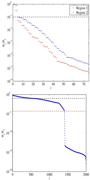
4.1 Normalized singular values of region 2. . . 52

4.2 Normalized singular values (Top) delay LM (Bottom) original LM. . . 53

4.3 Frequency Response. . . 54

4.4 Energy functions of (top)S11 and (bottom)S13 . . . 56

4.5 Normalized singular values (top) Proposed method (bottom) LM without delay extraction. . . 57

4.6 Comparaison of Proposed method and LM with the Data forS11. . . 58

4.7 Comparaison of Proposed method and LM with the Data forS13. . . 59

4.8 Three-port circuit of example 3 . . . 60

4.9 Energy functions of (top)Y11and (bottom)Y23 . . . 62

extraction. . . 63

4.11 Comparaison of Proposed method and LM with the Data for Y11 (a) and (b);

andY23(c) and (d) . . . 65

4.12 Comparaison of Proposed method and LM with the Data for Y11 (a) and (b);

andY23(c) and (d) . . . 66

3.1 Poles and Residues of the TF for Example 1 . . . 38

3.2 Comparison of poles RVF versus RVF-QRIV after the twentieth iteration . . . . 38

3.3 Error comparisons for original and modified data . . . 41

4.1 Poles, Residues and Delays of the TF . . . 51

4.2 Calculated poles and residues compared with theoretical values . . . 51

4.3 Time Axis Partitioning of (ω, τ) Plane of Example 2 . . . 51

4.4 Estimated delays versus optimized delays for Example 2 (Times inns) . . . 52

4.5 Results of the Rational Approximations of Example 2 . . . 55

4.6 Time Axis Partitioning of (ω, τ) Plane of Example 3 (Times inns) . . . 61

4.7 Estimated delays versus optimized delays for Example 3 (Times inns) . . . 64

4.8 Results of the Rational Approximations of Example 3 . . . 64

s Laplace variable (jω).

ω Angular frequency.

j Imaginary number.

τ Time Delay.

t Time.

∈ Belongs to.

|.| Absolute value.

arg[] Principal argument.

P Cauchy principal value.

IFFT Inverse fast Fourier transform.

LM Loewner matrix.

MNA Modified nodal analysis.

ODE Ordinary differential equations. PDE Partial differential equations. RVF Relaxed vector fitting.

SNR Signal-to-noise ratio.

VF Vector fitting.

Introduction

1.1

Background and Motivation

As the operating frequencies of high-speed electrical networks continue to increase, the

is-sue of signal propagation has taken a more prominent role in the design cycle. This increase

in operating speed has made the analysis of interconnects a major part in the design cycle of

electronic systems since previously neglected effects (Fig. 1.1) such as delay, crosstalk and attenuation can greatly affect the signal propagation on interconnects and the overall perfor-mance of electronic systems [1, 3]. The process of analysis, design, and validation of the

interconnect necessary for the successful transmission of signals is called signal integrity [4].

Because, interconnects exist at various levels in the design of any electronic systems such as

on-chip, packaging structures, printed circuit boards (PCB) and backplanes, interconnects are

considered to be the cause of the majority of signal degradation in the high-speed electronic

systems [1, 3, 5].

Simulating interconnect with circuit elements can be done using circuit simulators such as

SPICE [6], however in order to use these simulators, electrical models of the interconnects

Figure 1.1: Interconnect effects [1]

need to be done. Depending on the physical interconnect structure, signal rise times, and

the operating frequency of the circuit, different models can be used [1]. Developing analyti-cal interconnect models for the case when there are process variations, non-uniformities and

complex geometries is a challenging task, since analytical models require a full solution of

partial differential equations (PDE) which are hard to solve by circuit simulators. Analysis of distributed transmission lines when nonlinear elements are present give rise to the so-called

mixed frequency/time problem [1]. This problem arises from the fact that circuit simulators solve time-domain (transient) analysis using ordinary differential equations (ODE), while the PDE are traditionally solved in the frequency-domain. To overcome this problem,

macromod-eling techniques are used to convert the interconnect models into ODE.

Under these conditions, the behavior of interconnects lumped with other electromagnetic

mod-ules such as vias, connectors, and packages is often characterized by tabulated data, obtained

by measurements or by electromagnetic simulations [1, 3, 7–9]. Using inverse fast Fourier

transform (IFFT) [10] to convert the frequency-domain data into time domain data, analysis

of port responses can be computed by using convolution [11, 12]. Using IFFT directly on

the frequency-domain data can lead to inaccurate transient simulation [13, 14]. Another

ap-proach seeks to approximate the tabulated frequency data as a set of ODE, which can then be

easily incorporated with circuit simulators directly or converted into equivalent circuit, using

techniques referred as macromodel synthesis [1], the process of building mathematical models

important issue for the analysis of high-speed circuits.

Macromodeling of distributed networks characterized by frequency-domain data, is usually

performed using rational curve fitting techniques [1,3,7–9,15,16]. Among these techniques, the

Vector Fitting (VF) algorithms [9, 15–17] have emerged as a popular system identification tool

since the rational approximation is formulated as a linear least squares problem and relies on an

iterative pole relocation approach to improve the approximation. This leads to better numerical

stability and robustness when compared to non-iterative or polynomial approaches. In recent

years, Loewner Matrix (LM) [18, 19] has been proposed as an alternative to VF. Unlike, what

is done in VF, which relies on multiple different order approximations to determine the best order to fit the data [20], LM provides a direct mechanism to identify the order based on the

magnitudes of a Singular Value Decomposition (SVD) [18]. Furthermore, for the case of

multi-port networks the time-domain macromodel can be realized with fewer state space equations

when compared to VF [18, 19].

1.2

Objectives

Interconnect models derived from tabulated data are often used to obtain macromodels and

interact with SPICE circuit solvers [1, 3, 7–9, 15, 16].

The objective of this thesis is to develop efficient macromodeling algorithms for high-speed distributed networks by expanding on the known techniques. These algorithms do not make

any assumption about the underlying structure of the devices under study. Using only tabulated

frequency-data such as Y or S parameters obtained using measurements or by electromagnetic

simulations to characterize the networks. The methods developped in this work seek to address

specifically two issues: noisy tabulated data and tabulated data obtained from long distributed

1.3

Contributions

The main contributions of this thesis are:

1. A method is proposed to efficiently macromodel large multiport networks characterized by noisy frequency domain data. The method uses the concept of instrumental variable

[21, 22] to minimize the biasing effect of the least squares caused by the noise present in the data samples leading to more accurate solutions in fewer iterations.

2. Delayed rational approximations from tabulated frequency data are derived using the

LM method [18]. The method uses explicit delay extraction to extract propagation

de-lays estimates and partitions the data into single delay regions using a time-frequency

transform.

3. From the partitioned regions, a new approach to refine the delay estimates using the LM

method is performed.

4. The delay extraction LM algorithm is extended to multi-port networks. Numerical

exam-ples are presented to illustrate efficiency of the proposed method compared to traditional Loewner where the delays of the transfer function are not extracted.

1.4

Organization of the Thesis

The organization of the thesis is as follows. Chapter 2 offers an overview of different macro-modeling based on tabulated data, along with some of the issues related to these methods

and some of the state-of-art proposed solutions. Chapter 3 presents an efficient method to macromodel large multiport systems characterized by noisy frequency domain data, using a

of the pole-residue estimates with less iteration when compared to the traditional vector

fit-ting method. Chapter 4 presents a method to obtain delay rational macromodels of electrically

long interconnects from tabulated frequency data. Numerical examples are presented to

illus-trate efficiency of the proposed method compared to traditional Loewner where the delays are not extracted beforehand. A summary of the work presented along with suggestions of future

Literature Review

2.1

Overview

As mentioned in the previous chapter, due to system complexity, process variations and

non-uniformities of electrical circuits, rational macromodel approximations from tabulated

mea-sured data are often used to model high speed interconnects.

Among these techniques, the Vector Fitting (VF) algorithms [9, 15–17] have emerged as a

pop-ular system identification tool since the rational approximation is formulated as a linear least

squares problem and relies on an iterative pole relocation approach to improve the

approxima-tion. This leads to better numerical stability and robustness when compared to non-iterative or

polynomial approaches.

Although the VF method works well in estimating rational transfer functions, this is not the

case when dealing with large multi-port networks or when data samples are contaminated by

noise. Over the years, several modifications have been proposed to improve computational effi -ciency and accuracy of this method. To efficiently calculate the transfer functions of multi-port

networks using a common set of poles, a QR decomposition method was proposed to decouple

least squares equations of each transfer function [17]. The QR decomposition approach was

also used to implement a parallel processing VF algorithm for large multi-port networks [2].

Another issue with VF is that it has difficulty estimating the poles of transfer functions when data sample measurements are contaminated by noise. This is due to the fact that the noise of

the data causes the least squares solution to bias the location of the poles.

Various enhancements have been proposed to deal with noisy data, such as pole adding and

skimming method [23], least squares weighted functions [24] and instrumental variable VF

method [25], these method will be discussed in detail later in this chapter.

In recent years, Loewner Matrix (LM) [18, 19] has been proposed as an alternative to VF.

Un-like, what is done in VF, which relies on multiple different order approximations to determine the best order to fit the data [20], LM provides a direct mechanism to identify the order based

on the magnitudes of a Singular Value Decomposition (SVD) [18]. Furthermore, for the case

of multi-port networks the time-domain macromodel can be realized with fewer state space

equations when compared to VF [18, 19].

When dealing with long interconnects, attempting to approximate the tabulated data as rational

functions, will typically require many poles to accurately approximate the data [13, 29–31].

For distributed networks with long delays, methods based on delayed rational functions can

be used to provide accurate and efficient macromodels [13, 30, 31]. These techniques extract the propagation delays from the tabulated data, while the remaining attenuation losses are

approximated using low order rational functions, leading to more compact macromodels with

fewer poles when compared to using only rational functions.

In the following sections an overview of two popular rational curve techniques, vector fitting

(VF) and Loewner matrix (LM) are presented, along with some of the issues that can be

2.2

Vector Fitting

Using an iterative approach, the vector fitting algorithm allows to obtain a rational function to

approximate a set of tabulated data obtained either by measurement or electromagnetic

sim-ulation. It was originally introduced in context of analysis of transmission lines and power

systems, but was later extended to many fields, with signal integrity being among them.

Using the vector fitting algorithm, the objective is to approximate a set of tabulated data

(sk,Y(sk))K_k=1to get a rational function of the form

f(s)=

N X

n=1 cn

s− pn

+d+ se (2.1)

where pn and cn correspond to poles and residues respectively, these quantities can either be

real or complex conjugates, while the real variables d and e are optional; s is the Laplace

variable and Y(sk) is the value of the data at the particular k frequency. N is the order the

rational function.

VF is an iterative method that seeks to solve for the unknowns pn,cn,dande. This nonlinear

problem (because of the term pn that appears in the denominator) is solved by making into

a linear problem following a two stage process: 1) pole identification followed by 2) residue

identification.

Pole and Residues Identification

In the first stage, the goal is to obtain an approximation for the poles pn. This is done by

          

σ(s)f(s)

σ(s)

           =            PN n=1

cn

s−p¯n +d+se PN

n=1 ˜

cn s−p¯n +1

           (2.2)

where the terms ¯pn are starting values for the poles and the rest of the remaining terms are

unknown.

Multiplying the second row of (2.2) with f(s), the following relation is obtained

N X

n=1 cn

s− p¯n

+d+se=(

N X

n=1 ˜ cn

s− p¯n

+1)Y(s) (2.3)

Doing so, results in a linear problem where the unknowns arecn,c˜n,dande. Equation (2.3) for

a frequency point skgives a system of equation of the form

Akx= bk

where

Ak =           

Re(qk

1) . . . Re(q

k

N) 1 0 Re( ¯q k

1) . . . Re( ¯q

k N)

Im(qk

1) . . . Im(q

k

N) 1 0 Im( ¯q k

1) . . . Im( ¯q

k N)           

x= [c1 . . . cN d e c˜1 . . . c˜N]T (2.4)

bk =           

Re(Y(sk))

Depending on whether the poles are real or complex, the terms of (2.4) will have different forms, to make sure that the residues are either real or come in complex conjugate form. For

the case of real poles, the coefficients of (2.4) will be

qk_i = 1 sk− p¯i

¯

qk_i = −Y(sk) sk− p¯i

And for the case of complex poles the coefficients of (2.4) will become

qk_i = 1 sk− p¯i

+ 1

sk− p¯i+1 qk_i+1 = j

sk− p¯i

− j

sk− p¯i+1 ¯

qk_i = −Y(sk) sk −p¯i

+ −Y(sk)

sk− p¯i+1 ¯

qk_i+1 = −jY(sk) sk− p¯i

+ jY(sk)

sk −p¯i+1 ci =Re(ci) ci+1 =Re(ci)

˜

ci =Re(˜ci) c˜i+1 =Re(˜ci)

Expanding equation (2.4) forKfrequency points gives an overdetermined system of equations

From there the solution forxcan be obtained by doing

x=(ATA)−1(ATb) (2.5)

The least squares solution obtained from (2.5) can be used to get approximations for theσ(s)

andσ(s)f(s) functions written as

σ(s)f it = N Y

n=1

(s−z˜n)

(s− p¯n)

(2.6)

(σY)f it(s)= N Y

n=1

(s−zn)

(s− p¯n)

Finally from (2.6) an approximation for f(s) can be obtained as

f(s)=

N Y

n=1

(s−zn)

(s−˜zn)

(2.7)

It can be seen from equation (2.7), that the poles of f(s) become the zeros ofσ(s)f it. Therefore,

by taking the newly calculated zeros ofσ(s)f it as the new guess for the poles, this procedure

can be repeated until the poles converge.

In the procedure described above, it can be seen that only the zeros of the function σ(s)f it

are needed to first compute the poles. Once that is done, an additional least square solution,

corresponding to the second stage, is needed to obtain the residues and the termsdandeif they

2.2.1

Fast Vector Fitting

Although the VF method works well in estimating rational transfer functions, this is not the

case when dealing with large multi-port networks. Over the years, several modifications have

been proposed to improve computational efficiency and accuracy of this method. To efficiently calculate the transfer functions of multi-port networks using a common set of poles, a QR

decomposition method can be used to decouple least squares equations of each transfer function

[17].

Assuming a set of data coming from a multiport system{sk,Yj(sk)}K_k=1, where j= 1. . .J

corre-sponds to the number of transfer function in the transfer function matrix. For a system withP

number of ports,J = P2. The objective is to find the function

fj(s)= (σH

j_)(s)

σ(s) =

PN n=1

c_nj

s−pn +d+se PN

n=1 ˜

cn s−pn +1

(2.8)

such that f(sk)≈Y(sk). The terms c j

n,d,e,c˜n are unknown coefficients and ¯pn are chosen

heuristically in the first iteration. Using the same reasoning that was applied in the

previ-ous section, the solution for the J number of unknown equations (2.8) corresponds to solving

                            

X 0 0 0 −H1_X

0 X 0 0 −H2_X

. . . .

0 0 0 X −HJ_X                                                                   C1 C2 . . . CJ Cp                                      =                             

H1_1ˆ

H2_1ˆ

. . .

HJ_1ˆ                              (2.9) where

H0j = [Yj(s1). . .Yj(sK)],

Hj = diag([Re(H0j)Im(H0j)]), ˆ

1= (2K x1) column vector of one,

X0 =                     1

s1−p1 . . .

1

s1−pN

. . . .

1

sK−p1 . . .

1

sK−pN                     , X=           

Re(X0)

Im(X0)

          

andCj _{contains the residuesc}j

n andCp contains the residues ˜cn. The procedure is the same as

is done when dealing with a single transfer function, once the system is solved, the zeros of

σ(s)f it denoted z = {z1, . . . ,zN} become the poles of fj(s). The process is repeated again by

making{p1, . . . ,pN}= {z1, . . . ,zN}until convergence.

It was noted in [17] that since the residuescnj are discarded while convergence is not reached,

way that only the residues ˜cn are solved for, thus making the overdetermined set of equations

smaller. This is done by using the QR decomposition as described next.

Each j-th transfer function can be expressed as

[X −HjX]

           Cj Cp           

= Qj           

R₁₁j R₁₂j

0 R₂₂j                       Cj Cp           

Where the right hand side of the equation is the QR decomposition. Then by combining the

the factorization of all the matrices, the reduced set of equations where only the coefficientsCp

are the unknowns

                    R1 22 . . . RJ 22                    

Cp=                    

(Q1₎T_H1_1ˆ

. . .

(QJ₎T_HJ_1ˆ                    

Finally the solution is

Cp = J X

j=1

[(R₂₂j )TR₂₂j ]−1 J X

j=1

(QjR₂₂j )THj1ˆ (2.10)

Once the poles solution converges, the residues are solved by using what is done for the single

transfer function case. A visualization summary of the fast vector fitting algorithm can be seen

Figure 2.1: Application of QR on Multiport Networks [2].

2.2.2

Vector Fitting with Noisy Tabulated Data

One issue with VF is that it has difficulty estimating the poles of transfer functions when data sample measurements are contaminated by noise. This is due to the fact that the noise of the

data causes the least squares solution to bias the location of the poles. Various enhancements

have been proposed to deal with noisy data, such as relaxed vector fitting [15], pole adding

and skimming method [23], least squares weighted functions [24] and instrumental variable

VF method [25]. These techniques are briefly presented in the next sections.

Relaxed Vector Fitting

In [15], a change is made the original vector fitting algorithm, where the weight functionσ(s)

σ(s)=

N X

n=1 ˜ cn

s− p¯n

+c˜0 (2.11)

using this newσ(s), equation (2.2) becomes

N X

n=1 cn

s− p¯n

+d+se= (

N X

n=1 ˜ cn

s− p¯n

+c˜0)Y(s) (2.12)

Using this new form, (2.4) is now expressed at each frequency samplesk as

Ak =           

Re(qk₁) . . . Re(qk_N) 1 0 Re( ¯qk₁) . . . Re( ¯qk_N)

Im(qk

1) . . . Im(q

k

N) 1 0 Im( ¯q k

1) . . . Im( ¯q

k N)           

x= [c1 . . . cN d e c˜0 c˜1 . . . c˜N]T (2.13)

bk =            0 0           

where the terms are similar to what they were in the original form the vector fitting algorithm,

however since now bk is now equal, in order to avoid the trivial null solution, the following

equation is added

Re{ K X

k=1 (

N X

n=1 ˜ cn

s− p¯n

Using a similar approach as the previous section an overdetermined system of equation is

obtained and the rest of the algorithm is the same as the original vector fitting. This new

approach is often called relaxed vector fitting, and has been shown to have better properties

when the tabulated data is contaminated by noise, since it can improve the reallocation of the

poles [15]

Pole Adding and Skimming Method

In [20], another way to deal with rational approximation of data contaminated by noise using

vector fitting is presented. The method identifies so-called spurious poles which are said to

be responsible for the possible non-convergence of the standard vector fitting with noisy data.

These spurious poles are dealt with in a two step process, first they are identified and then

removed. In addition to dealing with noise, the method also presents a way to estimate the

order of the underlying system by incrementally increasing the number of poles and applying

relocation whenever it is necessary. The called is referred to in the paper as vector fitting

with adding and skimming (VF-AS) by the authors. The spurious poles are said affect the convergence of the vector fitting method, since they will tend be stuck at a specific location

and thus will never go to a better value at each subsequent iteration, indeed rather than trying

to fit true data, these spurious poles try to fit the noise instead. Another way of looking at

it, would be to consider that the constraint condition of (2.12) is not strong enough to for the

spurious poles to converge to their expected location.

In order to address this issue and enhance the convergence of the poles, a hard relocation is

proposed. This is a process through which an automatic detection of the spurious poles is

done. Then, the poles are placed in a location of the complex plane that is closer to the true

poles. Since VF is sensitive to the initial guess of the solution, it is expected that a better guess

Least Squares Weighted Functions

In [24], another modification to the standard vector fitting algorithm, when fitting data

con-taminated by noise, is proposed. In this method, the noise is assumed to be colored additive

with a zero-mean circular complex Gaussian distribution. The proposed method, uses

infor-mation about the variance of the data samples obtained with the use of least-squares weighting

functions. Estimation of the variance is done by performing measurements on a point-by-point

basis and is incorporated in the weighting function of vector fitting algorithm as

w(s)= 1

σ2_(s) (2.15)

Quality information of the data samples is then given to the least-squares estimator using the

weighting functions (2.15). This helps reduce the effect of the noise by improving the retrieval of the real behavior of system under study [24]

Instrumental Variable Vector Fitting

This section presents another modification to the vector fitting algorithm, when the tabulated

data is contaminated by noise. First, a more detailed look at how the nosy data samples can

bias the solution of the poles.

Consider the noisy tabulated data set defined as [25]

ˆ

whereY(s) is the exact transfer function andεis a zero-mean complex noise. In the presence

of noise, the system to be solved is modified and new terms are introduced due to the noise,Ak

andbk are replaced by

ˆ

Ak = Ak+HkA

ˆ

bk =bk+Hkb (2.17)

where the extra termsH_kAandH_kB are due toεand are defined as follows [25]:

H_kA =           

0 · · · 0 Re(˜ek₁) · · · Re(˜ek_N)

0 · · · 0 Im(˜ek₁) · · · Im(˜ek_N)

          

Hb_k =           

Re(εk)

Im(εk)            (2.18)

In the presence of noise the least square solution of (2.5) becomes:

x= "

X

k

ˆ AT_kAˆk

#−1" X

k

ˆ AT_kbˆk

#

(2.19)

ˆ

ATkAˆk = ATkAk+ATkH A k +(H

A k)

T

Ak +(HkA) T

HkA

ˆ

AT_kbˆk = ATkbk+ATkH b k +(H

A k)

T

bk+(HkA) T

H_kb (2.20)

the first termsAT

kAk andA T

kbk of (2.20) would be the terms found if there was no noise. Since,

as it was stated previously it is assumed that the disturbanceεis a zero-mean complex random

noise (meaning the expected mean value E[ε] is zero), the expected values of the second and

third terms in (2.20) are

E[ATkH A

k]=E[(H A k)

T

Ak]=0

E[AT_kH_kb]= E[(H_kA)Tbk]=0 (2.21)

the results in (2.21) mean that the second and third terms do not statistically bias the results of

(2.19). The fourth terms are defined as [25]

(HkA) T

HkA =[h a m,n]

(H_kA)THb_k =[hbm] (2.22)

ham,n=                         

Re(˜ek

m0)∗Re(˜ek_n0)+Im(˜ek_m0)∗Im(˜ek_n0),

m,n> N+2

0, otherwise

hbm=                         

Re(˜ek_m0)∗Re(εk)+Im(˜ekm0)∗Im(εk)

m> N+2

0, otherwise

(2.23)

withm0 = m−(N+2) andn0 =n−(N+2). Since the expected mean values ofE[Re(ε)2_{] and} E[Im(ε)2_{] are not equal to zero, we get the following}

E[(HkA) T

HkA], 0

E[(H_kA)TH_kb]_, 0 (2.24)

this means that the nonzeroha

m,n terms will bias the ˆA T

kAˆk matrices, thus affecting the solution

of all unknown variables in (2.19). The nonzero hb

m terms bias the residues which are used

to determine the poles of H(s). This biasing effect of hb

m is the main reason for the failure

of vector fitting to capture the actual poles of the system in the presence of zero-mean noise.

Next a technique to deal with least squares bias using the concept of instrumental variables is

presented.

X = "

X

k

ΨT kAˆk

#−1" X

k

ΨT kbˆk

#

(2.25)

whereΨkis called the instrumental variable, just as ˆAk was defined from the noisy data ˆY(s)=

Y(s)+ε,Ψk = Ak+H_kΨis also obtained from a set of data ˆY(s)=Y(s)+ρ. Note that in both sets,

Y(s) is the same theoretical noise free transfer function andεandρare uncorrelated Gaussian

noise.

Using the definition ofΨ, the terms in (2.19) become:

ΨT

kAˆk =ATkAk+ATkH A

k +(HkΨ) T

Ak +(HkΨ) T

H_kA

ΨT

kbˆk = ATkbk +ATkH b

k +(HkΨ) T

bk+(HkΨ) T

Hb_k (2.26)

The first three terms of (2.26) have the same values as those in (2.20), the only difference is in the fourth term. Since the values of the Hk terms come from the noise in the data sets and we

are dealing with uncorrelated noise, the expected value of the fourth term also becomes zero

when using the instrumental variable approach, leaving the least square solution with only the

no-noise terms [21, 22, 26–28].

E[(H_kΨ)TH_kA]=0

2.3

Loewner Matrix

The Loewner Matrix method [18] seeks to macromodel the transfer functionY(s) as

Y(s)=C(sE−A)−1B+D+sY∞ (2.28)

whereA,E ∈ _Rn×n,B ∈ _Rn×1,C ∈ _R1×n,D ∈ _R,Y∞ ∈ _Rdescribe the system of ordern. The

descriptor state space matricesA,B,C,andEare obtained as follows.

First the given data is split into two groups, usually referred to right and left interpolation data

points as

[s1. . .sK]=[µ1. . . µk]∪[λ1. . . λk]

[Y(s1). . .Y(sK)]=

[Y(µ1). . .Y(µk)]∪[Y(λ1). . .Y(λk)]

wherek+k= Kand

              

k= k= K/2 ifKis even k= k+1= (K+1)/2 ifKis odd

There are many ways that the data could be split. In this work, the alternating splitting of

in [18, 19]. V=                     v1 ... vk                     =                    

Y(µ1)

...

Y(µk)                     , W=

w1. . .wk

=Y(λ1). . .Y(λk)

With the left data set (µi,vi) and right data set (λi,wi), thek×kLoewner and Shifted Loewner

matrices are computed as follows

L=                    

v1−w1

µ1−λ1 . . .

v1−wk

µ1−λ_k

... ... ...

vk−w1

µk−λ1 . . .

vk−wk

µk−λ_k                     (2.29)

σL=

                   

µ1v1−λ1w1

µ1−λ1 . . .

µ1v1−λkwk

µ1−λ_k

... ... ...

µkvk−λ1w1

µk−λ1 . . .

µkvk−λkwk

µk−λ_k                     (2.30)

Once the Loewner and shifted Loewner are computed, the next step is to determine the order

of the approximation. In order to do that, a singular value decomposition (SVD) is performed

on (sL−σL). Any value of scan be chosen as long as it is not the eigenvalue of the (σL,L)

SVD(sL−σL)= [Y,Σ,X] (2.31)

whereΣis a diagonal matrix containing the singular values. The ordernof the approximation is

chosen as the location where a large drop of the normalized singular value happens as described

in [18, 19]. The descriptor system matrices are constructed as

A=−Yn∗σLXn, B= Yn∗V, (2.32)

C=WXn, E=−Yn∗LXn

whereXn∈Rk×nandYn∈ Rk×nare constructed from the firstncolumns ofXandYof (2.31)

respectively [18, 19].

The method presented above leads to strictly proper rational approximations (i.e.DandY∞ _is

equal to zero). However, for the case when it is required to useDandY∞_{, setting these terms}

to zero may lead to unstable and inaccurate macromodels as illustrated in [19]. In this work,

if the LM approximation produces unstable poles, the D andY∞ _{terms are extracted by first}

extracting the stable poles of the system, these will constitute theA,E,B,Cmatrices. As for

theDandY∞_{terms, they are obtained by fitting the remaining unstable poles using a first order}

2.4

Macromodeling Data from Long Interconnects

Depending on the type of structure under study, different approach exists for developing macro-models of distributed networks. When dealing with long interconnects, attempting to

ap-proximate the tabulated data as rational functions, will typically require many poles to

ac-curately approximate the data [13, 29–31]. For distributed networks with long delays, methods

based on delayed rational functions can be used to provide accurate and efficient macromod-els [13, 30, 31]. These techniques extract the propagation delays from the tabulated data, while

the remaining attenuation losses are approximated using low order rational functions, leading

to more compact macromodels with fewer poles when compared to using only rational

func-tions. The next sections presents a summary of the different techniques that have been proposed to deal with tabulated data that describe the behavior of distributed networks with long delays.

2.4.1

Delay-Extraction Macromodeling using Hilbert Transforms

In [13, 14], a delay extraction based techniques using the Hilbert transform is presented. The

method uses the concept of minimum phase functions for passive structures to obtain a delay

estimate of the distributed networks. A function that has all its poles and zeros in the left-half

plane is called a minimum phase function [32], in multi-port stable networks, this property is

only present in diagonal elements. Considering a network of the following form

Y(s)=[Yi j(s)] (i, j∈1, . . . ,P) (2.33)

system can be written as product of a minimum phase function and an all-pass function as

Yi j(s)=Yi jmin(s)Y AP

i j (s) (2.34)

whereY_{i j}min(s) is the minimum phase function part andY_{i j}AP(s) is the all-pass portion, the Hilbert

transform can be used to extract the delay and the attenuation losses part (function

correspond-ing to the delay-free part of the function) as follows.

Equation (2.22) can be rewritten in following form

Yi j(s)= Yˆi j(s)e−sτ (2.35)

where ˆYi j(s) is the delay-free portion and e−sτ is the delay part portion corresponding to the

extracted delayτ. The equivalence of (2.22) and (2.23) stems from the fact thate−sτacts as an

all pass function since|e−sτ_| = _{1 (|}._{|corresponding to magnitude), leaving the delay-free term}

ˆ

Yi j(s) correspond to the minimum phase function. The first step of the delay-extraction based

on Hilbert transform is to get an estimate for the delay termτ. This can be done by rearranging

(2.23) to obtain an expression for the unknownτterm as follows [13, 14, 32]

τ=−Average Slope arg "

Yi j(s)

ˆ Yi j(s)

#!

(2.36)

wherearg(z) refers to the principal argument of a complex number z. In order to computeτ,

|Yˆi j(s)|=|Yi j(s)| (2.37)

arg[ ˆYi j(s)]= −HT{ln|Yi j(s)|} (2.38)

In (2.26)HT{.}stands for the Hilbert transform [32], using the discrete Hilbert transform [32],

(2.26) can be rewritten as [13, 14]

arg[ ˆYi j(s)]=−

1 2πP

Z π

θ=−π

ln|Yi j(θ)|cot

ω−θ

2

!

dθ (2.39)

wherePdenotes the Cauchy principal value of the integral that follows. Once (2.39) is solved,

τis obtained from (2.36). This allows to get all the off-diagonal terms as a product of minimum phase functions and an all-pass functions.

2.4.2

Compact Macromodeling of Electrically Long Interconnects

In [33], a method for macromodeling long interconnects is introduced. Starting from

frequency-domain scattering data, the technique produces compact macromodels based on multiple delay

extraction and rational approximations.

Using a set of measured frequency samples denoted as

fork =1, . . . ,K, the goal is to find a rational approximation of the form

H(s)= X

m

Qm(s)e−sTm (2.40)

whereTm represents the signal propagation delays andQm(s) represent effects such as

attenu-ation losses and dispersion. Using the technique, first the number of delays is truncated to a

finite number ˜m and second a rational approximation is applied to eachQm(s). The resulting

delayed rational model is

H(s)' ˜

m X

m=1

Rm0+Pnn¯=1

Rmn s−an

r0+Pnn¯=1

rn s−an

e−sτm _(2.41)

where τm ' Tm are suitable estimates of the dominant propagation delays, and an is a set of

poles. It can be seen that when ˜m= 1,Tm˜ = 0, (4.21) becomes a normal rational approximation modeled like the regular vector fitting. The first stage of the identification of (2.41) is to

identify estimates of dominant delay termsτmfor the tabulated data. This is done with a

Time-Frequency transform called the Gabor transform [34]. Details of how it is used to identify the

delays will be presented in chapter 3. Once the set of dominant delays is known, what is left is

the estimation of the coefficientsRmn,rn of (2.41). This can be done in the same as the normal

Modeling Noisy Multiport Networks

In this chapter, the Instrumental Variable Vector Fitting method covered in section 2.1.2 is

com-bined with the QR Decomposition technique of section 2.1.1 to efficiently macromodel large multiport networks characterized by noisy frequency domain data. The instrumental variable

method is used to minimize the biasing effect of the least squares caused by the noise present in the data samples leading to more accurate solutions in fewer iterations. Furthermore, for

the case of multiport networks described by common poles, the QR decomposition proposed

in section 2.1.1 is used to decouple the equations which reduces the overall computation time

and memory requirements for calculating the transfer functions. It is illustrated that the

com-bination of the Instrumental Variable approach with QR decomposition leads to a lower errors

and faster convergence of the overall macromodel when compared to using vector fitting with

QR decomposition only (Fast vector fitting).

3.1

Problem formulation and review

As with it was done in section 2.1.2, consider tabulated frequency data from measurements

ˆ

Y_kj =Y_kj+ε_kj

where Y_kj is thek-th data sample of the j-th transfer function in the absence of noise and ε_kj

is the zero-mean complex random noise perturbing the k-th data sample of the j-th transfer

function. The system of equations for the j-th transfer function can be expressed as

[X −Hˆ jX]

           Cj Cp           

= _Hˆj_ˆ

1 (3.1)

whereCj corresponds to the unknown residues for the j-th transfer function, whileCp

corre-sponds to the coefficients used to compute the unknown common poles shared among all the transfer functions describing the multiport network. A detailed description of the termsX, ˆHj

and ˆ1can be found in section 2.1.1 of the second chapter.

When trying to fit a multiport network with M transfer functions (i.e j = 1, . . . ,M) using common poles for all the transfer functions, the system of equations using (3.1) are coupled

due to the shared coefficients of Cp. To improve the efficiency of VF, a QR decomposition

method is used to decouple the system of equations, which lead to simplified set of equations

that depend only on Cp [17]. For this purpose, QR decomposition is applied to the left half

side of (3.1) for each j-th transfer function

[X −HˆjX]= Qˆj            ˆ

R₁₁j Rˆ₁₂j

Next by combining the factorization of all the matrices, the following reduced set of equations

is obtained, where only the coefficientsCpare the unknowns

                    ˆ R1₂₂

. . .

ˆ R₂₂M

                   

Cp =                    

( ˆQ1)THˆ11ˆ

. . .

( ˆQM)THˆM1ˆ                     (3.3)

Since (3.3) is an overdetermined system, its least squares solution forCpis expressed as

M X

j=1

[( ˆR₂₂j )TRˆ₂₂j ] Cp =

M X

j=1

( ˆQjRˆ₂₂j )THˆ j1ˆ (3.4)

In order to examine how the noise biases the least squares solution of (3.4), the terms ˆHj, ˆR₂₂j

and ˆQjRˆ₂₂j , are written as

ˆ

Hj = Hj+N_hj ˆ

R₂₂j = R₂₂j +N_rj_ε ˆ

QjRˆ₂₂j = QjR₂₂j +Nqjε (3.5)

whereHj_,Rj

22andQ

j_{terms are derived fromY}j

k, if the data samples had no noise, andN j h,N

j rε

andNqjεare due to the errorε j

k in the data samples. Since, the noisy termsN j h,N

j

rεandN j qεare

( ˆQjRˆ₂₂j )THˆ j = (QjR₂₂j )THj+(QjR₂₂j )TN_hj

+(N_qj_ε)THj+(N_qj_ε)TN_hj ( ˆR₂₂j )TRˆ₂₂j = (R₂₂j )TR₂₂j +(R₂₂j )TN_rj_ε

+(Nrjε) T

R₂₂j +(Nrjε) T

Nrjε (3.6)

Note that (Qj_Rj

22)

T_Hj _{and (R}j

22)

T_Rj

22of (3.6) are the matrices obtained in the absence of noise. Since it is assumed that the biasing of the noise is zero (i.e. expected mean value,E[ε] = 0), the expected values of the second and third terms on the right-hand side of (3.6) are also zero.

Thus, these terms do not statistically bias the results of the least squares approximation. For

the fourth terms on the right hand side of (3.6), their expected values do not equal to zero,

since they are the product of two correlated matrices. Therefore, it is due to the biasing effect of (Nqjε)TN

j

hand (N j rε)TN

j

rε, that (3.4) fails to capture actual poles of the system in the presence

of zero-mean noise.

For the implementation of the relaxed VF algorithm (RVF) [15], it can be shown that the noise

also bias the least squares solution [25]. However, because the right hand side of (3.3) does

not include ( ˆQj₎T_Hˆ j_{1ˆ when implementing RVF, only the ( ˆR}j

22)

T_Rˆj

22 terms end up biasing the solution. This contributes to RVF being able to obtain more accurate results when compared

to VF.

3.2

Proposed Algorithm

M X

j=1

[( ˜R_IVj ₂₂)TRˆ₂₂j ] Cp =

M X

j=1

( ˜Q_IVj R˜_IVj ₂₂)THˆ j1ˆ (3.7)

where the terms ˜Q_IVj and ˜R_IVj ₂₂come from a QR decomposition performed on the j-th transfer

function of the system X− Ψˆ j_{X. The term ˆ}Ψj _{is constructed from di}ff_{erent data estimates,}

ˆ

Y_IVkj =Y_kj+η_kj, whereη_kj is the error of approximation ofY_kj and is assumed to be a zero mean noise uncorrelated withε_kj. Since the terms ˜R_IVj ₂₂and ˜Q_IVj R˜_IVj ₂₂are formulated from a different set of noisy data samples, they can be expressed similar to (3.5), withNrjη andN

j

qη due to the

errorη_kj in the data samples.

Next, to investigate the biasing effect of the noise, the product terms of (3.7) for the j-th transfer function are expressed as

( ˜Q_IVj R˜_IVj ₂₂)THˆ j = (QjR₂₂j )THj+(QjR₂₂j )TN_hj

+(N_qj_η)THj+(N_qj_η)TN_hj ( ˜R_IVj ₂₂)TRˆ₂₂j = (R₂₂j )TR₂₂j +(R₂₂j )TNrjε

+(N_rj_η)TR₂₂j +(N_rj_η)TN_rj_ε (3.8)

Since it is assumed that the biasing effect ofεandηare zero, the expected mean values of the second and third terms of the right hand side of (3.8) are zero. Furthermore, since it is assumed

that ε and η are uncorrelated to each other (i.e. E[η_kjε_kj] = 0), the expected mean values of the fourth terms are also zero. As a result, by using a different approximation uncorrelated to the original data, the instrumental variable provides a statistically unbiased result to the least

In this work, the previous rational approximation of the VF method is used to create the data

samples of ˆY_IVkj = Y_kj + η_kj, similar to the approach described in [25]. Since the errors of the previous rational approximation is less correlated to the errors of the original data, it is

demonstrated in Section IV that this yields better rational approximations without significantly

increasing the complexity of the VF method.

3.3

Numerical Example

3.3.1

Synthetic Transfer Function

As a proof of concept, a transfer function (TF) with known poles and residues described in

Table 3.1 with added noise is approximated. The TF is contaminated with a white gaussian

noise with a signal to noise ration (SNR) of 35 dB. the TF is sampled using 2000 evenly

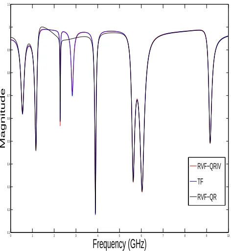
spaced point that range from 0 to 10 GHz. A rational approximation is performed using the

classic VF algorithm and the proposed method, the resulting approximations are compared

with the original noiseless TF in Fig. 3.1. It can be seen that contrary to the VF algorithm,

which cannot capture all the poles, the VF-IVQR method captures all 16 poles of the original

TF. A second rational approximation is also performed with a SNR of 25 dB. Instead of using

the classic VF, the algorithms are performed using the relaxed version of VF [15]. Once again,

as it can be seen in Fig. 3.4, the QR fails to capture all the poles as accurately as

RVF-IVQR. Along with the TF approximations, RMS Error versus the number of iterations plots

are also provided for VF and RVF in Fig. 3.2 and Fig. 3.3 respectively. Table 3.2 provides

a comparison between the RVF-QR and the RVF-QRIV poles, the proposed method has very

low error when compared to the original poles of the TF, compared to the RVF-QR which has

a relatively high percentage error in one of the pole, this error gets even greater when using the

0 1 2 3 4 5 6 7 8 9 10 0.1

0.2 0.3 0.4 0.5 0.6 0.7 0.8 0.9 1

Frequency (GHz)

Magnitude

VF−QRIV TF VF−QR

Figure 3.1: Rational approximations of the 35 dB SNR data.

2 4 6 8 10 12 14 16 18 20

0 0.05 0.1 0.15 0.2 0.25 0.3 0.35

Iterations

RMS Error

VF−QR VF−QRIV

2 4 6 8 10 12 14 16 18 20 0

0.05 0.1 0.15 0.2 0.25 0.3 0.35

Iterations

RMS Error

RVF−QR RVF−QRIV

Figure 3.3: RMS Error versus iteration count for SNR=25dB.

0 1 2 3 4 5 6 7 8 9 10

0.1 0.2 0.3 0.4 0.5 0.6 0.7 0.8 0.9 1 1.1

Frequency (GHz)

Magnitude

RVF−QRIV TF RVF−QR

Table 3.1: Poles and Residues of the TF for Example 1

Poles (GHz) Residues (GHz)

d =0.98

−0.6132± j3.4551 −0.9877∓ j0.0809

−0.3940± j7.3758 −0.2067∓ j0.0131

−0.0880± j14.3024 −0.1382∓ j0.0145

−0.4097± j17.7864 −0.1182∓ j0.0166

−0.2991± j24.4622 −0.2426∓ j0.0145

−0.6447± j35.2669 −0.4043∓ j0.0297

−1.0135± j37.9655 −0.6787∓ j0.1465

−0.5711± j57.4748 −0.2626∓ j0.1037

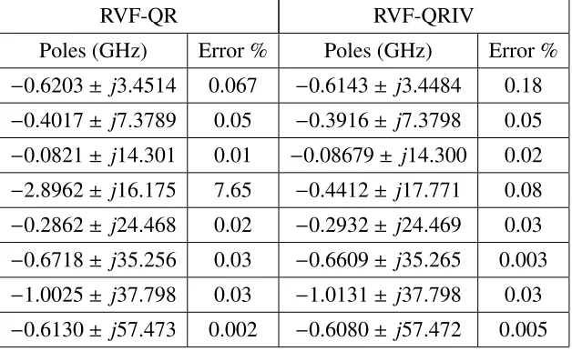
Table 3.2: Comparison of poles RVF versus RVF-QRIV after the twentieth iteration

RVF-QR RVF-QRIV

Poles (GHz) Error % Poles (GHz) Error %

−0.6203± j3.4514 0.067 −0.6143± j3.4484 0.18

−0.4017± j7.3789 0.05 −0.3916± j7.3798 0.05

−0.0821± j14.301 0.01 −0.08679± j14.300 0.02

−2.8962± j16.175 7.65 −0.4412± j17.771 0.08

−0.2862± j24.468 0.02 −0.2932± j24.469 0.03

−0.6718± j35.256 0.03 −0.6609± j35.265 0.003

−1.0025± j37.798 0.03 −1.0131± j37.798 0.03

−0.6130± j57.473 0.002 −0.6080± j57.472 0.005

3.3.2

Four Port Network

A four port network of a two differential pairs of Strada-Whisper connectors is characterized in terms of the S-parameters measured using a vector network analyzer. A circuit description

of the four port network is provided in example 3 of [25]. Since this is a four port

symmet-ric network, ten transfer functions are fitted simultaneously using 100 common poles. The

data is fitted using VF [9], instrumental variable VF (VF-IV), relaxed VF (RVF) [15] and

QR decomposition algorithm. The initial guess of the poles is distributed evenly among the

imaginary axis as complex conjugate poles between 0 to 12 GHz. Fig. 3.5 shows normalized

H2-norm [18] for 10 iterations which measures the error in the magnitude of all the entries of

the S-parameter matrix. The instrumental variable was created after the first iteration for the

IV algorithms. A sample of the rational approximation forS13for RVF and RVF-IV, is shown

in Fig. 2.

It should be noted that the difference between the macromodels obtained from VF, VF-IV, RVF and RVF-IV is dependent on the level of noise in the data. For high signal-to-noise ratio (SNR),

all methods will give similar results. In the proposed VF-IV and RVF-IV, the biasing effect due to (8) is reduced since the noise matrices (using the instrumental variable approach) are less

correlated. For this example, RVF, VF-IV and RVF-IV were able to get capture the transfer

functions. Nonetheless, VF-IV and RVF-IV converged faster and achieved lower error (Fig.

3.5). As the noise of data sample increases, the instrumental variable will tend to outperform

the VF and RVF due to the reduced biasing of the least squares solution. To illustrate this point,

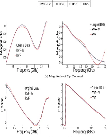
the noise obtained bySi j−Sjiis multiplied by five and ten and added toSi j. Table 3.3 compares

the error after the tenth iteration for original and modified data. In addition, zoomed regions of

S13(for noise multiplied by ten) are shown in Fig. 3 to show that the RVF-IV performs better

than RVF. Since all four methods rely on QR decomposition to decouple the least squares

equations, their CPU times were close to 9 seconds using an Intel Xeon dual-processor (3.16

GHz) and 4 GB of RAM. In comparison to [25], which does not decouple the equations of

2

4

6

8

10

0.09

0.095

0.1

0.105

0.11

Iterations

H

2

Error

VF

VF−IV

RVF

RVF−IV

Figure 3.5: NormalizedH₂-norm versus number of iterations.

0

2

4

6

8

10

12

0

0.05

0.1

0.15

0.2

0.25

Frequency (GHz)

Magnitude

Noisy Data RVF−IV RVF

Table 3.3: Error comparisons for original and modified data

H₂-norm

Method Original 5x 10x

VF 0.108 0.120 0.134

RVF 0.091 0.095 0.100

VF-IV 0.086 0.086 0.086

RVF-IV 0.086 0.086 0.086

0.5 1 1.5 2 2.5 3

0.02 0.04 0.06 0.08 0.1

Frequency (GHz)

Original Data

RVF−IV

RVF

10.8 11 11.2 11.4 11.6 11.8 12

0.01 0.02 0.03 0.04 0.05 0.06 0.07

Frequency (GHz)

Original Data

RVF−IV

RVF

(a) Magnitude ofS₁₃Zoomed.

0 0.5 1 1.5 2 2.5

0 0.5 1 1.5

Frequency (GHz)

Original Data

RVF−IV

RVF

10.5 11 11.5 12

−3 −2 −1 0 1 2 3

Frequency (GHz)

Original Data

RVF−IV

RVF

(b) Phase ofS13Zoomed.

Delay Extraction Loewner Method

4.1

Introduction

Methodologies to obtain delayed rational functions have been proposed in [30, 35] using the

VF approach for the attenuation losses approximations. However, these delayed rational

func-tion techniques have not been extended to the LM approach. In this chapter, delayed rafunc-tional

approximations from tabulated frequency data are derived using the LM method, based on the

concepts developed in [36]. The method uses explicit delay extraction to extract propagation

delays estimates and partitions the data into single delay regions using a time-frequency

trans-form. A new approach to refine the delay estimates for each partitioned region is also proposed

using the LM method. Once the best delay estimates are identified, the LM method is used

to obtain rational approximations for each region. The developed delay extraction LM

algo-rithm is also applied to multi-port networks. Numerical examples are presented to illustrate

efficiency of the proposed method compared to traditional Loewner where the delays of the transfer function are not extracted.

4.2

Macormodels with Delays and Review of General

Time-Frequency Decomposition

4.2.1

Theoretical Motivation

The main objective of the proposed method is to produce a delayed rational function of the

following form:

Hi j(s)= M X

m=1

H_{i j}(m)(s)e−sTm _(4.1)

whereTmis themthpropagation delay andH

(m)

i j (s) is the delay free rational approximation

cor-responding tomth delay. In practice, it is possible to approximate a long interconnect without

the extraction of the delay terms, however this generally results in a very high number of poles,

which makes the transient analysis computationally intensive. By extracting the delay, the

at-tenuation losses can be approximated by low order rational function [13,14,29–31,35,37]. The

next section presents an overview of estimating the delays when dealing with electrically long

distributed networks characterized by measured or simulated data.

4.2.2

Time-Frequency Decomposition

The delay extraction is done using the concept of the time-frequency decomposition

trans-forms. A time-frequency transform relatesHi j(s) toFi j(ω, τ) with the following relation:

Fi j(ω, τ)= ∞ Z

−∞

whereW(ζ−ω) is a window centred atζ = ωof specific width L[34, 38] It is observed from (4.2) that if W = 1, then the equation becomes the standard definition of the Inverse Fourier Transform (IFT). Therefore the time-frequency transform can be thought of as an IFT ofHi j(s),

that only retains the frequency components in the frequency band of the filtering windowW.

In this work, the Gabor transform [34, 38] is used, since it provides optimal support in both the

time and frequency domain. The energy contents ofFi j(ω, τ) over time is obtained by,

ηi j(t)= ∞ Z

−∞

|Fi j(ω, τ)|2dω (4.3)

where the propagation delays can be identified as the local maxima of theηi j(t) function [30].

The inverse of (4.2) is defined as [34, 38]:

Hi j(ζ)=

1 2π

∞

"

−∞

Fi j(ω, τ)W(ζ−ω)e−jωτdωdτ (4.4)

Using (4.3), the reconstruction ofHi j(ζ) can be done by splitting the time-frequency plane into

separate regionsΩmand performing the integral (4.4) over each region as follows [29, 30]

Hi j(ζ)= X

k e H_{i j}(m)(ζ)

e

H(_{i j}m)(ζ)= 1 2π

"

Ωm

Fi j(ω, τ)W(ζ−ω)e −jωτ

dωdτ (4.5)

[

m

Ωm= R2

The summation of each integral of (4.5) leads to the reconstruction of Hi j(ζ). The

distributed networks characterized by measured or simulated data.

4.3

Proposed Algorithm

Once the delays are determined from the measured data, the proposed work approximates

the attenuation losses corresponding to each delay using a Loewner matrix approach. The

steps involved are identifying of most significant propagation delays, partitioning of the

time-frequency plane in regions and performing rational approximation of the attenuation losses

using Loewner matrix.

4.3.1

Estimation of Propagation Delays and Partitioning Regions

The first step of the proposed algorithm is to estimate the propagation delays, given the

tab-ulated data Hi j. The time-frequency representation Fi j(ω, τ) is computed using (4.2). Once

the time-frequency plane is obtained, evaluating the energy content over timeηi j(t) using (4.3)

provides estimates of the propagation delays, as the time values of the local maxima [30].

In order to extract the most relevant delays, all delay terms with relative energy contributions

below a user-chosen toleranceεare not taken into account

ˆ n(_{i j}k) X

k

ˆ n(_{i j}k)

where ˆn(_{i j}k)is the energy content of a local delay evaluated as [30]

ˆ

n(_{i j}k) = 1 2π

Z τk

τk−1

ηi j(τ)dτ (4.7)

whereτk−1 andτk correspond to local minimums between thekth local maximum of the

func-tionηi j(τ). The value ofεis problem dependent and is chosen such that the energy contribution

of the neglected delays does not significantly affect the accuracy of the model [30, 31].

Once the estimated delays are identified, the next step is to split the time-frequency plane in

such a way as to get delay regions. The method used to split the plane is the same as the one

proposed in [30, 31]. The partitioning for the (ω, τ) plane intoΩmis done by choosing a point

tk between adjacent delaysTk andTk+1, where the value of the energy content at that point is lower than a predefined valueδ

ηi j(τ=tk)< δ (4.8)

Using (4.7), regions Ωm are defined to be regions between two adjacent minima tk and tk+1, expressed as follows:

Ωm∈ {(ω, τ) : 0≤ω ≤2πFmax, tk ≤τ≤tk+1} (4.9)

Depending on the value of the estimated delay computed using the time-frequency transform,

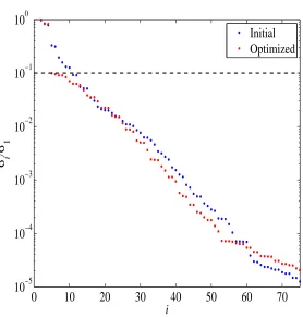
the order of the rational approximation that is chosen is not always optimal, therefore an extra

reduce the order of the rational function of each regionΩi. In this work, the delay optimization

is performed using a similar method to what is done in [37], however, instead of using the error

of the rational approximation for different delay values, the optimized delay is determined by considering the normalized singular values drop obtained from the SVD of the Loewner matrix.

Details of how to select the optimized delay which leads to a low order rational approximation

will be provided once LM method is presented.

4.3.2

Estimating Attenuation Losses

H

(

s

)

Once theΩm regions are determined, the last step involves computing the attenuation losses

rational function corresponding to each region. There are two cases that can arise when

es-timating attenuation losses; regions where there is only one identified delay peak in Ωm and

regions where there are more than one identified delay peak present inΩm.

For the case where there is only one identified delay peak, the goal is to evaluate

˜

H_{i j}(m)(s)≈ H_{i j}(m)(s)e−sTm _(4.10)

whereTmis the known extracted delay and ˜H( m)

i j (s) is obtained using (4.5).

To get the rational approximation H_{i j}(m)(s) for each region, the frequency domain data is

ex-pressed as

{sk,H˜( m)

i j (sk)e