Active Power Dispatch Optimization for a Grid-Connected Microgrid with Uncertain Multi-Type Loads

Article

Active Power Dispatch Optimization for a

Grid-Connected Microgrid with Uncertain

Multi-Type Loads

Kai Lv, Hao Tang *, Yijing Li and Xin Li

School of Electrical Engineering and Automation, Hefei University of Technology, Hefei 230009, China; [email protected] (K.L.); [email protected] (Y.L.); [email protected] (X.L.)

* Correspondence: [email protected]; Tel.: +86-551-6290-1416

Abstract: An active power dispatch method for a microgrid (MG) with multi-type loads, renewable energy sources (RESs) and distributed energy storage devices (DESDs) is the focus of this paper. The MG operates in a grid-connected model, and distributed power sources contribute to the service for load demands. The outputs of multiple DESDs are controlled to optimize the active power dispatch. Our goal with optimization is to reduce the economic cost under time-of-use (TOU) price, and to adjust the excessively high or low load rate of distributed transformers (DTs) caused by the peak-valley demand and load uncertainties. To simulate a practical environment, the stochastic characteristics of multi-type loads are formulated. The transition matrix of system state is provided. Then, a finite-horizon Markov decision process (FHMDP) model is established to describe the dispatch optimization problem. A learning-based technique is adopted to search the optimal joint control policy of multiple DESDs. Finally, simulation experiments are performed to validate the effectiveness of the proposed method, and the fuzzification analysis of the method is presented.

Keywords: multi-type loads; active power dispatch optimization; simulated-annealing Q-learning

0. Nomination

N

number of nodes

M

number of loads

U

number of RESs

C

number of DESDs

L

Y

position matrix of load

R

Y

position matrix of RES

S

Y

position matrix of DESD

L

p

active power vector of load

R

p

active power vector of RES

S

p

active power vector of DESD

N

p

active power vector

N n

p

active power consumed on node

n

N

P

active power flow matrix

W

TOU price

Tr

O

capacity matrix of DT

Tr

2 of 20

*

L

upper limit of ideal load rate range

*

L

lower limit of ideal load rate range

L m

U

basic pu value of load m



L m

U

predicted value of load m

Δ L

m

U

variation value of load m



m

h

ratio of Δ L( )

m

U t and ULm( )t m

h

level of



h

m

L m

p

maximum demand of load m

L m p

minimum demand of load m L

O

basic value vector of load

R

O

capacity vector of RES

R v

U

basic per-unit value of RESs

c

SOC

SOC of DESD

c

c

DE

self-discharge proportion of DESD

c

S

O

capacity matrix of DESDs

cs

E

maximum SOC level of DESD

c

c

e

SOC level of DESD

c

l

D

low price periods

m

D

moderate price periods

h

D high price periods

1. Introduction

1.1 MG and active-power dispatch optimization

3 of 20

1.2 Difficulties and solutions

In this paper, we assume the control centre observes the system state and makes dispatch decisions at discrete times. The control problem of multiple DESDs is modelled as a finite horizon Markov decision process (FHMDP), which is a common model in stochastic dynamic programming [7]. To make a proper decision, the control centre should collect a variety of information at each decision epoch, such as the time-of-use (TOU) price, the current load at each node and the outputs of each RES. This means that the state space will expand geometrically when the operation information is transformed into system state, which is the "curse of dimensionality" problem [8]. Applying the traditional numerical optimization algorithm (e.g., policy iteration) to this optimization problem will be difficult due to the expanding dimensionality of the system state. Furthermore, it is difficult to build an exact model of the MG system due to the complexity of the system and stochastic dynamics. This "curse of modelling" problem will be more obvious when the influence of model parameters error is considered.

To solve these difficulties, we first choose the most essential state components to reduce the state-space dimension and simplify the system model. As TOU price and RES output are correlated to time, we replace the TOU price and RES output states with a time state to reduce one dimensionality of state space, instead of considering TOU price and RES output as state components. Secondly, we introduce a reinforcement learning (RL)–based method to solve the optimization problem. RL is a machine learning algorithm which is an online optimization and model-free method [9]. During the optimization process of RL, action explorations under each state can yield a variety of samples, with which the necessary state-action values can be learned and a better control policy can be found. This process can be realized by observing the operation of an actual MG system without an exact system model. Finally, a simulated annealing method is adopted in this paper to construct the exploration scheme, which is efficient for avoiding local optima.

1.3 Related works

MG technology can provide high efficiency and flexible access to the integration and utilization of RES and DESD. In recent years, a large amount of research has been performed concerning dispatch optimization for MGs.

In dispatch optimization for MGs, economic dispatch has become vital and mostly accessible with the wide applications of electricity price technologies (e.g., real-time price, TOU). The TOU price mechanism is increasingly applied in daily life, which can lead to grid consumption a better state [10]. Considering the relationship between TOU price and economic dispatch for MGs, a key observation is that MG can achieve economic benefits from the operation of units inside only if the TOU price difference among different grid operation periods exceeds economic losses of units in [11]. According to this observation, the problem of optimal dispatch for the MG under TOU is solved [12]. A demand-side energy management system for a grid-connected MG with forecasted loads is developed in [13], where the responsive behaviours of customers under TOU are modelled by a matrix of self-elasticity and cross-elasticity. With the application of a genetic algorithm, the active power flow is optimized by multiple DESDs control in [14] and TOU cost management program is tested.

4 of 20

MG by the control of DESD is studied in [21]. In [22], an optimal dispatch method for a multi-region MG is proposed, where the variation processes of multiple loads are described by a discrete time Markov model, and long-term interaction currents between the MG and external grid are reduced by the control of multiple DESDs.

In this paper, besides economic dispatch, another goal of active power dispatch optimization is to adjust the unexpected load rate of distributed transformers. Load rate of DT is defined by the ratio of the total peak load to its capacity. In reality, the load rate is a key factor affecting the service life of a transformer, which varies continuously. Considering annual load rate, a method for predicting and monitoring the service lifetime of DT is presented in [23]. Supposing the capacity of DT is determined, an algorithm for calculating the optimal load rate of DT is proposed in [24]. Although it is important for DT and network operation, there is little consideration of the load rate adjustment for DT when the dispatch optimization problems are solved. Therefore, with concern for economy improvement and load rate adjustment, we study a dispatch optimization problem for the MG.

Among the dispatch optimization studies for MGs, several algorithms are used to solve the “curse of modelling” and “curse of dimensionality” problems. Considering uncertainties of RES and electric vehicle (EV) load in the MG, schedule optimization for the charging process of EVs is presented in [25], where the Simulation-based Policy Improvement (SBPI) method is adopted to solve the “curse of modelling” problem. An approximate dynamic programming technique is adopted in [26] to solve the “curse of dimensionality” occurring in the energy dispatch optimization for the MG with thermo-electric load and RES. However, these two algorithms are not suitable for this work due to the number of the samples that SBPI needs increasing geometrically as the state space expands, and the application of ADP technique adopted in [26] to this work needs the exact model of the MG. The algorithm that we use to solve the optimization problems is associated with simulated-annealing Q-learning (SAQ) [27], in which the simulated annealing is introduced in Q-learning algorithm to balance exploration and exploitation. SAQ will avoid not only the curse of modelling and the curse of dimensionality but also the local optima problem, which often occurs with Q-learning.

1.4 Main contributions

In this paper, a dispatch optimization method for the grid-connected MG is proposed to minimize the economic cost and adjust the load rates of DTs. To establish a more practical model, the stochastic characteristics of multi-type loads are discussed. The contributions of this paper can be summarized as follows:

• We consider a general approach to model the active-power dispatch of the MG with RES, DESD

and load, in which the numbers and positions of units (e.g., RES, DESD) can be set adaptably.

• We describe a stochastic dispatch model for the MG using a finite-horizon markov decision

model, where the uncertainties of multi-type loads and the adjustment for load rate of DT are

considered.

• We adopt a SAQ method to solve the dispatch optimization problem, and the method can

perform online learning optimization.

The remainder of this paper is organized as follows. In section 2, we describe the architecture of the MG with multi-types loads. In section 3, we formulate the problem into FHMDP mathematically. In section 4, we present the SAQ algorithm for the dispatch optimization problem. We provide simulation results in section 5 and some brief conclusions in section 6.

2. The physical model of MG

5 of 20

regular load or provide power as a generator unit. We assume that the MG network consists of N nodes. M loads, V RESs and C DESDs connect to these nodes dispersedly.

Let L =[ ₁L,..., L,..., L]τ∈ N M×

n N

Y Y Y Y R be the position matrix of load, where

=[ (1),..., ( ),..., ( )]

L L L L

n n n n

Y Y Y m Y M consolidates the information of the loads connecting to node

n

,

satisfying

( ) 0 ,

1 ,

L

n

if load m connect to node n Y m

otherwise 

=



(1)

Similarly, let R( )

n

Y v and S( )

n

Y c be the element consolidating the information of the RES

v

and DESD c connecting to node

n

respectively, and denote R =[ R(1),, R( ),, R( )]

n n n n

Y Y Y v Y V ,

=[ (1),..., ( ),..., ( )]

S S S S

n n n n

Y Y Y c Y C , R =[ ₁R, ₂R,..., R]τ ∈ N V×

V

Y Y Y Y R and S =[ ₁S, ₂S,..., S]τ ∈ N C×

N

Y Y Y Y R .

Let L( )

m

p t be the active power demand of load

m

at time t , and denote

τ

= 1

( ) [ ( ),..., ( )]

L L L

M

p t p t p t

∈

R

M×1. Similarly, let R( )

v

p t be the active power output of RES

m

, S( )

c p t

be the active power output of DESD

c

and denote = ∈ ×1

1

( ) [ ,..., ,..., ]

R R R R V

v V

p t p p p R ,

×

= ∈ 1

1

[ ,..., ,..., ]

S S S S C

c C

p p p p R . We assume that the RESs do not consume power and the loads do not

provide power in this work, which implies that the elements of R( )

p t are non-positive and the

elements of S( )

p t are non-negative. As opposed to these two units, DESD can make a bi-directional

power transfer with outside environments. When DESD

c

charges, S( )

c

p t is positive, and S( )

c p t is

negative when DESD

c

discharges. The power consumed on node

n

consists of the power from

the units connected to the node, so the active power vector N( ) [= ₁N,..., N,..., N]τ

n N

p t p p p satisfies

( ) L L( ) ( ) ( )

N R R S S

Y p t Y p t Y p

p t = + + t

(2)

From Equation (3) and (4), it is observed that the vectors L, R, S

p p p and N

p can be obtained if

information about all units in the MG is known. Then, all the active power flow information of the

MG can be obtained. We describe the structure of node

n

to introduce the working mode of each

node in the MG.

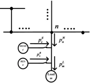
Figure 1 Structure diagram of node

n

Figure 1 shows the structure diagram of node

n

. The active power consumed on node

n

at

time t can be expressed as follows:

= ( )+ ( )+ (

) )

( L L R R S S

n n n n

p t Y p t Y p t Y p t

(3)

τ τ

η ( N( ) ( ))= ( ( ) ( ))η + ( )

N N n N

N P t e n e n P t p t

(4)

6 of 20

11 1 1

1

1

( ) ... ( ) ... ( )

( ) ... ( ) ... ( )

( )

( ) ... ( ) ... ( )

N N N

q N

N N N

N N N

n nq nN

N N N

N Nq NN

P P P

P P P

P

P P P

t t t

t t t

t R

t t t

×

 

 

 

 

=_{ }∈

 

 

 

 

    

    

(5)

η

N is a row vector with each element equal to 1 and

e n

( )

is a column unit vector with the n-th

element equals to 1 and others equal to 0.

Without loss of generality, we let node 1 be the external power grid and PCC is located between

node 1 and node 2. We denote

W t

( )

as the TOU price at time t and the economic cost between t

and t+ Δt can be calculated as

+Δ +Δ

Δ =



=





1

( , ) t t{ ( ) * ( )} t t{ ( ) * N( )}

e _t G _t q

q

f t t W t P t dt W t P t dt

(6)

In addition to the economic cost, another type of information about the MG which we focus on is the load rate of DT as mentioned in section 1. Load rate has a large impact on DT, so the two types of unexpected load rates mentioned in section 1 are attempted to be avoided. The capacity matrix of

transformers in the MG is denoted as N N

Tr

O ∈R × with element O n q_Tr( , ) being the rated capacity

of DT located between node

n

and node

q

, and the power factor matrix of DT is denoted as

N N Tr

F ∈R × with element F n q_Tr( , ) being the power factor of DT located between node

n

and node

q

. We assume that O n x_Tr( , ) and F n x_Tr( , ) are∞ if there is no transformer between node

n

and

node

x

. The matrix O_Tr depends on the network structure of the MG, which has no correlation

with the state of the devices. From O_Tr and Equations (3) and (4), the load rate matrix L_Trcan be

calculated as follows:

[ ( ]

( ) )

Tr T

N

r Tr P t

L t = ∅F ∅O

(7)

in which ∅ denotes element-wise division operation.

The ideal range of the load rate of DT is denoted as [ , ]L L* * . When L_Tr( )t is calculated, we can

determine the operation quality of DTs by comparing the non-zero elements in L_Tr( )t with the

upper bound

L

* and lower bound

L

*. As excessively high or low load rates will have adverse

effects on DT and L_Tr is uncontrollable for a structure-known MG, we can change

P

N and N

p to adjust the load rate of DTs according to Equation (6).

The goal of dispatch optimization is to reduce the economic cost of the MG and adjust the unexpected load rate of DTs. As in most cases, the maximum power point of RES is expected to be traced and the load demand should be met in this paper. Therefore, we control the output of DESDs in each period when required to change the active power flow in the MG network. The control

actions are defined by =( ₁S, ₂S,..., S)

C

a p p p , where p_cs is the output power of DESD

c

. During peak

periods, DESDs can provide energy for the MG to ease the supply pressure. On the other hand, the charging action of DESD in the valley period can improve the low power-demand level of the MG. However, considering the limited capacity of DESDs, there are two special cases as follows:

7 of 20

Case 2. The SOC of one DESD reaches the lower limit for discharging actions. Discharging operation to DESD is forbidden in this case, as the over-discharging operation would lower the performance of DESD.

As we focus on the daily dispatch for the MG in this work, we let T_B=0 andT_D =24. In the

following section, models of each component in the MG are discussed.

2.1 Multi-type loads

Normally, electricity load in daily life can be divided into three types: residential load, commercial load, and industrial load. In this paper, we consider the case that the loads in the MG consist of the residential load and commercial load. Figure 2 and 3 show the daily per-unit (pu)

profile of the commercial and residential load. In these figures, interval

a

denotes the difference

between the maximal load value and forecasted load value, and interval b denotes the difference

between the forecasted load value and minimal load value. As shown in the figures, the real-time value of load varies within an interval. These variations appear during each day because of the random behaviour of power consumers [28]. Considering this uncertain characteristic, we model the power demand with randomness in Figures 2 and 3.

Figure 2 Daily profile of the commercial load Figure 3 Daily profile of the residential load

Let O_L =[O_L(1),,O m_L( ),,O M_L( )] be the basic value vector of load in which O m_L( ) is

the basic value of the load m, UmL( )t be the pu value of load m,

L_{( )} m

U t be the predicted pu value

and ΔU tmL( ) be the variation value (pu). Then, for load

m

∈

{1,



,

M

}

, the load demand can be

expressed as follows:



( )

( ) *

( ) (

L

( )

( )) *

( )

L L L

m

m

t

U t O m

m L

U t

U t

m

O m

L

p

=

=

+ Δ

(8)

We let



*

( )

*

L

( )

L

m

m m

U t

h

U t

Δ

=

(

9

)

where L( )

m

p t is the maximum load value, p t_mL( ) is the minimum load value. Then, Equation (8) can

be translated into



*

( )

(1

_m

) *

Lm

( ) *

_L

( )

L

m

t

h

p

= +

U t O m

(10)

satisfying the following constraints:

( ) ( ) ( )

L L L

mt m t p tm p ≤p ≤

(11) 0

0.2 0.4 0.6 0.8 1 1.2 1.4

0 2 4 6 8 10 12 14 16 18 20 22 24

pu va

lu

e

time (h)

interval a interval b

0 0.2 0.4 0.6 0.8 1 1.2

0 2 4 6 8 10 12 14 16 18 20 22 24

pu va

lu

e

time (h)

8 of 20

( ) ( ) * ( )

L L

L m t U tm O

p = m

(12)

( ) ( ) * ( )

L L

L m t U tm O

p = m

(13)

Because _{is correlated to} O m_L( ) and it is non-random when O m_L( ) is set, the

randomness of load m can be viewed as the randomness of *

m

h . For each type of load, the predicted

load value ULm( )t and variation characteristic of h_m* vary. The predicted value of residential load

and commercial load at different periods[29-30] can be viewed as their basic values. The variation

characteristic of *

m

h is associated with time, the type of load m and environment conditions, which

can be modelled as a markov process and demonstrated by different state and transition probabilities [31].

2.2 DESD

Considering the charging and discharging efficiency, the SOC of DESD

c

∈

{1,..., }

C

in this

paper is calculated using Equation (14):

(

)

(

)

( ) / ( ) ( )

( ) ( ) , ( ) 0

( )

( ) ( ) ( )

( ) ( ) , ( ) 0

( ) S

t t _{c dis c S}

S

c c _t c

S S

t t _{c cha c S S}

c c _t c

S

p t t DE O c

SOC t t SOC t p t

O c

p t t DE O c

SOC t t SOC t p t

O c

η

η

+Δ

+Δ

 _{− ⋅}

 _{+ Δ = + ≤}

 

⋅ − ⋅



+ Δ = + >

 





(14)

The SOC of DESD c and the action to DESD c satisfy the following constraints:

≤ ≤ max

0 SOC t_c( ) SOC_c (15)

≤ ≥

( ) 0 ( ) upl

S

c c c

p t if SOC t SOC (16)

≥ ≤

( ) 0 ( )

S downl

c c c

p t if SOC t SOC (17)

Where

η

_dis and

η

_cha are the discharging and charging efficiency. DE_c and O c_S( ) are the

self-discharge power proportion and the nominal capacity of battery

c

. Moreover, the charging

action to DESD c is forbidden once the SOC reaches upl

c

SOC and the discharging action to DESD c

is forbidden once the SOC reaches downl

c

SOC .

We divide the SOC of DESD c into B_c intervals corresponding to B_c levels. B_c intervals can

be denoted as

−

max max max max

max

[0,

c

),[

c

,2

c

),...,[(

1) *

c

,

]

c c

c c c c

SOC

SOC

SOC

SOC

B

SOC

B

B

B

B

. Given SOC tc( )

andp t_c( ), the interval containing SOC t_c( + Δt) can be calculated by Equation (14) and the SOC

level at t+ Δt can be further known. Considering the two special cases of the action to DESD

mentioned in Section 1, the SOC information of DESDs should be observed at each decision epoch, so we denote the SOC level of DESDs as state components in the problem-solving process.

9 of 20

2.3 Distributed generation and TOU price

Figure 4 Daily profile (pu) of PV

In MGs, the RES usually includes photovoltaic (PV), wind power, etc. In this paper, we assume that the RESs in the MG are PV sources. If there are multi-type RES in the MG, the method in this work is still feasible with the model of each RES. The output of PV is the maximum at midday and is approximately symmetric in one day. Figure 4 shows the output value (pu) of a 450KW PV system during a 24-hour period, where the data can found in [32]. For a given PV system, we can approximately predict the output power during a certain time according to this curve and its capacity.

In this paper, the output of PV

v

at time t can be defined by

( ) ( ) ( )

R R

v t O v UR v

p = ⋅ t

(18)

Here, O_Ris the capacity vector of PV sources, where O v_R( ) is the capacity of the RES

v

, and

( )

R v

U t is the output value (pu) of RES

v

at time t . The mapping function from time to U_vR can be

expressed as follows:

=         

∈ ∈

∈ ∈

∈ ∈

∈ ∈

∈ ∈

∈

0 [0,4) [22,23]

0.2 [4,6) [18,22)

0.4 [6,8) [17,18)

0.6 [8,9) [16,17)

0.8 [9,11) [14,16)

1 [11,14)

( ) R v

t and t

t and t

t and t

t and t

t and t

t U t

(19)

We assume that the TOU price consists of three periods: high price period, moderate price period, low price period. The mapping function from time to TOU prices can be expressed as:

( )

R_low t D_l R_mid t D_m R_high t D_h

W t

=

    

∈ ∈

∈

(20)

From Equations (18-20), we can obtain the PV output and TOU price for each period once the TOU price scheme and capacity of each PV are known.

3. Mathematical model and optimization method

In this section, we formulate the dispatch optimization problem as a finite-horizon Markov decision process (FHMDP) with Markovian state transition. We model this problem as a FHMDP

due to the following reasons：

1. The natural uncertainties and randomness of the load and PV can be described by Markov

models as in numerous MGs and smart grid research [33-36].

2. Considering the effects of current actions to later system states, power dispatch of the power

system in a given period of time can be modelled by discrete-time finite-state Markov chains [37].

0 0.2 0.4 0.6 0.8 1

0 2 4 6 8 10 12 14 16 18 20 22 24

output

va

lue

10 of 20

The FHMDP can be described by the tuple<T S A P f, , , , >. To model the optimization

problem into FHMDP, we transform the continuous states and actions into discrete variables. Various components of the tuple and their discretization processes are described in detail as follows:

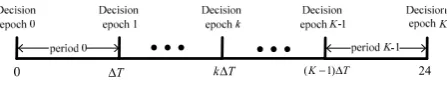
Figure 5 Decisionepoch and periods

Action and decision epoch: Figure 5 shows the decision epochs and operation periods of the

MG system. We denote a set of decision epochs as

T

=

{0,1,...,

K

−

1}

and the time duration of one

period is

Δ =

T

24

K

−1. The action chosen in decision epoch k∈{0,1,...,K−1} which will be

performed in the period k is denoted by ( )=( ₁S( ), ₂S( ),..., S( ))

C

a k p k p k p k ， where

∈ = ₁× × _c× × _C,

a A A A A A_c= −{ p_s,0, }, c {1,p_s ∈ ,C}. We assume p t_s( ) is constant when ∈[ *Δ , ( +1) *Δ )

t k T k T . There is no action at decision epoch K, when system reaches the

terminate state.

State: Denote state in period k as ( )=( , ₁( ),..., ( ), ( )₁ ,..., ( ))∈ = K× Lo

M

ad C

s k k h k h k b k b k S S S ×SBat,

where h k_m( ) represents the level state of h k_m( ) at period k and b k_c( ) denotes the SOC level

state of DESD

c

at period k. Let L = L1× ×... LM

S S S be the state space of the load variation level,

and D = D1× ×... DC

S S S be the state space of the level. The discretization process from *

( )

m

h k to

( ) m

h k is shown as follows:

First, the load-variation state is denoted as h_m( ) {k ∈ −Z_m,..., 1,0,1,...,− Z_m} . Then, we

discretize U k U k U kmL( ), Lm( ), _mL( ) and determine the value of these variables in each period as Figure

2 and Figure 3, where these values are constant in one epoch. The value of Δ L

m

U when h k_m( )=z

is defined by

   = −   _>   = =  Δ  _<   − ( ) ( ) ( ) , ( ) ( 0 ) (

( )| , 0

0 ) , m L L m m L L m m h L _L m _m k z

k U k z Z

U U k

U k k

z U z Z z k z U

(21)

Then, L( )

m

p k can be calculated by Equation (10), the output of RES

m

can be calculated as

Equations (18-19) and operation information of the MG is known once the action to multiple DESDs are chosen.

Transition:

P S A S

= × × →

[1,0]

represents the state transition function, which can be

described by the transition of the state component as follows:

The period state transition can be characterized by the state transition probabilityP k k_T( '| ),

satisfying

 = +

=

≠ +

 ,

1 , ' 1

( '| )

0 ' 1

T

k k k k P k k

(22)

k TΔ

T

11 of 20

The SOC state transition can be characterized by the state transition probability +

( 1)| ( ), ( )

( )

B bc bc

P k k a k . The SOC level changes over time depending on the actions taken. Therefore, we can calculate continuous SOC values as (14) and renew current SOC-level states at each decision epoch.

The load-variation state transition can be characterized by the state transition probability +

( 1)| ( )) ( _m

L m

P h k h k , which will be evaluated by estimating the variation given the current state

and load type. The transition of the load variation level state is independent of the transition of the SOC level state, so the overall state transition probabilities can be defined by

= =

+

=

×

∏

+

×

∏

+

1 1

(

1)| ( ), ( ))

( '| )

(

1)|

(

(

( ))

(

(

1)| ( ), ( ))

M C

T B m m L c c

m c

s k

s k a k

P k k

P

k

k

P

k

k a k

P

h

h

b

b

(

23

)

Cost function: The cost function consists of economic cost and load rate cost and is denoted as

( ) ( )

( ( ), ( )) _{e e} ( ), ( ) _{Tr Tr} ( ), ( )

f s k a k =

θ

f s k a k +

θ

f s k a k

(24) where

1 2

{1,..., } {1,..., } {1,..., } {1,..., }

( ( ), ( ))

( ( ), ( ))

( ( ), ( ))

Tr h ij l ij

i N j N i N j N

f s k a k

θ

y s k a k

θ

y s k a k

∈ ∈ ∈ ∈

=

 

+

 

(25)

= Δ

( ( ), ( )) ( ( )) * ( ( ), ( )) *

e G

f s k a k W s k P s k a k T (26)

In (22),

1 ( ), ( )

*

1

( , )

( ( ), ( ))

0

Tr s k a k

ij

L i j

y s k a k

else

L



_>



=





(27)

*

2

1 0

( , )

( ), ( )

( ( ), ( ))

0

Tr s k a k

ij

L i j

L

y s k a k

else



_<

_<



=





(28)

For FHMDP, the system obtains the terminate cost once the terminate state is reached. The terminate cost is correlated to the terminate state, and the terminate cost is defined by a function of SOC levels of multiple DESDs,

θ

=



( (

))

_g

e

_cs

(

)

g

s K

K

(29)

From Equations (22-25), we can see that values of

θ θ

_e, _TRH,

θ

_TRL will affect the optimization

process, and these values can be adjusted to realize various objectives such as solely economic

optimization with

θ

_TR =0. The control policy is denoted by

π

:

S

→

A

,

π

∈Ω

where Ω is the set

of the policy. The cost expected to be minimized is the average sum of each cost during the entire day, which can be defined by

π −

_π

=

=



1

+

0

[

( ( ), ( ( )))

( ( ))]

K

k

J

E

f s k

s k

g s K

(30)

The objective of the proposed method is to find an optimal policyπ* which minimizes the

average total cost of the MG during one day，that is

π π

π

∈Ω =

*

arg minJ

12 of 20

To find the optimal policy, we propose a SAQ based method according to the FHMDP model. SAQ is a typical reinforcement learning method, which can evaluate the expected utility of the available actions without a certain model of the environment. The method can effectively solve problems with stochastic transitions and costs. Additionally, SAQ can be implemented to solve optimization problems by simulating or observing a running system and learning the state-action value.

In SAQ, the Q-factor is denoted as

Q s k a k

( ( ), ( ))

and its updating function for FHMDP is

shown as Equations (32-33):

When the next state of

s k

( )

is a terminate state,k= −K 1,

( ( ), ( )) ( ( ), ( )) ( (s( ), ( )) ( ( ), ( )) ( ))

Q s k a k =Q s k a k +β f k a k −Q s k a k +αV K (32)

When it is not a terminate state,k ≠K-1,

*

( ( ), ( )) ( ( ), ( )) ( ( ( ), ( )) ( ( ), ( )) min ( ( 1), )) a A

s k a k

Q s k a k Q s k a k

β

f Q s k a k

α

Q s k a

∈

= + − + + (33)

In Equation (31),

V K

( )

is a function that depends on terminate state

s K

( )

. In this paper, we

define it by

ω

= ⋅ )

) (

( g s K( )

V K (34)

whereω is a coefficient.

The ε-greedy scheme is commonly used in Q-learning to trade off exploration and exploit.

However, geometrically expanding state space will make a great impact on the effect of ε-greedy

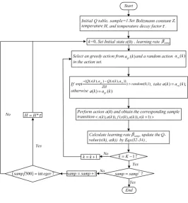
scheme. Therefore, we introduce simulated annealing to construct the exploration scheme. Detailed information about the algorithm can be acquired from the flow chart in Figure 6.

Figure 6 Flow chart of SAQ

4. Numerical results and analysis

In this section, we present several results to illustrate the effectiveness of the dispatch method proposed. Without loss of generality, we assume that the number of load at each node is 1 at most, as well as the number of RES and DESD. A MG system including commercial loads, residential

( ), ( )), ( ( ), ( )), ( 1)

s k a k f s k a k s k

< + >

(0)

s

1

samp samp= +

1

k k= + k= −K 1？

*

samp samp= ？

( ) gr

a k a krn( )

samp

β

samp

β

τ

( ( ( ), ) ( ( ), ))

exp( Q s k agr Q s k arn ) _random(0,1)

ZH

− −

> a k( )=a krn( ) ( ) gr( )

a k =a k

*

H=Hτ

13 of 20

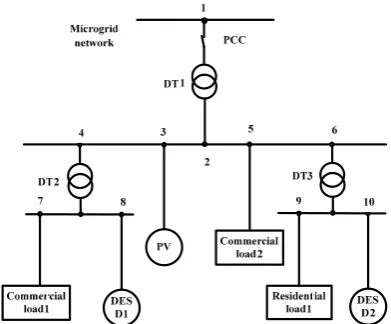
loads, PV, DTs and DESDs is shown in Figure 7. As the focus of this work is the active power dispatch, we assume that the power factor of each DT is 0.95. The basic value of commercial load 1 and 2 and residential load 1 are 120 KW, 90KW and 100KW, respectively, and their pu-values are shown in Figure 1 and Figure 2. The other parameters of the MG are as follows: parameters of DESDs are listed in Table 1. Nominal capacity and the limits of each DT are summarized in Table 2. Parameters involved in discretization and learning optimization are listed in Table 3. The price of different TOU mechanisms at each period is shown in Appendix A, which is used to make several comparisons with the proposed method.

Figure 7 Structure diagram of MG with multiple types of load

Table 1. Parameters of DESDs

η

dis

(%)

η

cha

(%)

c DE

(%)

( ) S O c

(KWh)

upl c

SOC downl

c SOC

DESD1 98 98 0.5 100 0.80 0.20

DESD2 97 97 0.7 80 0.75 0.25

Table 2. Parameters of DTs

Capacity

(KVA)

*

L

(%) (%)

DT1 300 100 40

DT2 120 100 40

DT3 100 100 40

Table 3. Parameters of SAQ

Parameter E1 E2 K Z1 Z2 θe θTr

θ

g

value 5 4 24 3 2 1 1 10

Parameter

θ

l

θ

h H Z τ

β

α

ω

value 40 100 10 1 0.95 0.96 0.98 40

*

14 of 20

Figure 8 Average economic cost curve Figure 9 Average load rate cost curve

Figure 8 and Figure 9 show the optimization curves of the average economic cost and load rate cost. From many repeated and independent runs, we observed that the SAQ usually finds a better policy than the Q-learning algorithm as shown in the figures above. With SAQ, the economic cost of the system is reduced by 25%, which is approximately 3% better than Q-learning. Additionally, we can observe that the optimization convergence rate is fast for both methods, but the fluctuations at the early stage are obvious in both. The fast convergence rate is due to some obvious and easily accessible transition laws for the controller, such as the transition laws of PV generation and TOU price, which only depend on the current decision epoch. The early fluctuation range is obvious because high price periods have a large impact on the average cost of the system, during which different policies will lead to large differences in the average cost. The load rate cost is reduced by approximately 80% more than the economic cost, but still cannot be eliminated completely. As the capacity of each DESD is limited, the DESDs are not able to assist in adjusting the load rate when the loads reach continuously low or high conditions. Therefore, the load rate cost still exists after optimization.

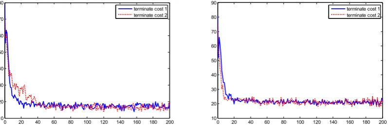
Figure 10 Economic cost under differentg s K( ( )) Figure 11 Load rate cost under differentg s K( ( ))

Figure 10 and Figure 11 show the average economic cost and load rate costs with different termination cost function g s K1( ( ))=

θ

_g*



( ( ))e K_cs and g s K2( ( )) -=

θ

_g*



( ( ))e K_cs . From the two figures above, we can obtain the following two conclusions.

First, when the terminated cost is 1

( ( ))

g s K , the convergence rate of economic cost is faster.

This occurs because when the termination cost is 1

( ( ))

g s K , the system can learn such a fact faster: It is advantageous to sell out the electrical energy at the last time in a day. As samples are mutually independent when we study a FHMDP problem, the energy stored in the DESDs

0 20 40 60 80 100 120 140 160 180 200

210 220 230 240 250 260 270 280 290

Q learning SAQ

early fluctuation

0 20 40 60 80 100 120 140 160 180 200

10 20 30 40 50 60 70 80 90

Q learning SAQ

early fluctuation

0 20 40 60 80 100 120 140 160 180 200

210 220 230 240 250 260 270 280

terminate cost 1 terminate cost 2

0 20 40 60 80 100 120 140 160 180 200

10 20 30 40 50 60 70 80 90

15 of 20

will not be used after the current day sample in this paper. This information will guide the smart control agent to sell the energy and decrease the economic cost.

Second, different than the economic cost, the convergence rate of the load rate cost is slower

when the termination cost is 1

( ( ))

g s K . In this case, the agent will learn quickly that it is advantageous to store a number of energy at later periods in the day. As the excessively low load rate mainly occurs at the valley periods, the charging actions of DESDs will increase the load rate of DTs effectively. Therefore, the load rate cost decreases quickly when the termination cost is

2

( ( ))

g s K and the economic cost decreases slowly.

Figure 10 and Figure 11 show that the definition of termination costs can affect the optimization process of the system to an extent. However, when the termination cost is defined differently, there is little difference in the final optimization results of each cost, although the convergence rates vary dramatically. This is due to that the effect of termination cost to optimization will decline as the optimization process undergoing and the agent will eventually learn the optimal policy irrespective of the termination cost. Termination cost is still important, especially considering the online optimization. For different systems and objectives in online cases, we can choose the corresponding termination costs to make the optimization process faster and more accurate.

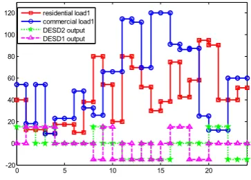
Figure 12 Active Power of each unit in one day

Figure 12 shows the power of loads and DESDs in a 24-hour sample where the MG system operates under the optimal policy. In this sample, the initial SOC of two DESDs are 0.202 and 0.157. The load demands are light in the MG between hours 1~7, at this time, DESDs store energy from the network within its power range to take advantage of the low-price periods. When the MG reaches the first middle-price duration, the actions of the DESDs vary. In hour 8, DESD1 takes a charging action to prepare for the peak-load and high-price periods, but DESD2 takes a discharging action to avoid the high load rate as the residential-load demand becomes high at this time. In hour 9, DESD1 takes an idling action as the SOC reaches the upper limit and DESD2 takes a charging action. Between hours 11~16, DESDs never take charging actions, as the TOU price is high and a peak-load period of commercial load appears at this time. DESD1 take discharging actions at hour 11, 12, 14 and 15 when the load rate of DT2 will be excessively high without the supply of DESD. The load rate will inevitably become high once the peak-load duration exceeds the maximal supply time of DESDs. For later periods, DESDs take charging actions once the load demands are excessively low, meanwhile the energy is sold out to decrease the economic cost given that the discharging will not cause an excessively low load rate.

0 5 10 15 20

-20 0 20 40 60 80 100

16 of 20

(a) (b)

(c) (d)

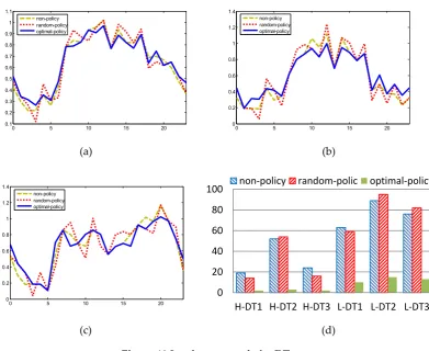
Figure 13 Load rate records for DTs

Figure 13 (a-c) shows the load rate record of DT 1-3 under three different policies. Non-policy indicates that DESDs take no actions irrespective of the solutions provided by the MG. At each decision period, random policy indicates that the DESDs select an action randomly in admissible action space. The load rate under non-policy demonstrates the inherent load-factor performance of the MG. (a) shows the load rate of DT1 in one day (one sample), which shows that the excessively low load rate occurring in night periods is regulated. In some samples, excessively low load rates still exist because of the uncertainty of the initial SOC and the duration of peak load periods, just like the early period in (b). Between hours 10 to 14, the power outputs of DESDs increase to decrease the load rate as the load demand in the MG rises in (c). (d) shows the statistical data of excessively high and low load rate within a month. H-DT1 is the number of periods when excessively high load rate occurs, and L-DT1 is the number of periods when excessively high load rate occurs. The regulation effect of high load rate is more obvious than the effect of low load rate, as excessively high load rates will cause more cost to the MG system.

Fig 14 Fuzzification results

0 5 10 15 20

0.1 0.2 0.3 0.4 0.5 0.6 0.7 0.8 0.9 1 1.1

non-policy random-policy optimal-policy

0 5 10 15 20

0 0.2 0.4 0.6 0.8 1 1.2 1.4

non-policy random-policy optimal-policy

0 5 10 15 20

0 0.2 0.4 0.6 0.8 1 1.2 1.4

non-policy random-policy optimal-policy

0 20 40 60 80 100

H-DT1 H-DT2 H-DT3 L-DT1 L-DT2 L-DT3 non-policy random-polic optimal-policy

0 50 100 150 200 250 300

0 0.2 0.4 0.6 0.8 1 1.2 1.4 1.6 1.8 2

θ

Tr

17 of 20

Moreover, the fuzzification result of the proposed method is presented in Figure 14, where we

let

θ θ

_e+ _Tr =2 . The objective of the dispatch will be economic optimization or load rate

optimization when

θ

_Tris 0 and 2. From the figure, the load rate cost under optimal policy when

=0 Tr

θ

is obviously lower than the cost under random policy when

θ

_Tr=2 because the actions for

economic dispatch simultaneously regulate the load rate to an extent in some periods, such as the discharging action at high-price periods, which are peak periods. On the other hand, the economic cost and load rate cost of the multi-objective dispatch model are slightly larger than those under single-objective dispatch. This shows that the multi-objective optimization method in this paper can find a variety of solutions for decreasing the load rate cost and economic cost to achieve DT security

and economic benefits. Therefore, for different MGs and controllers, the parameters

θ

_Trand

θ

_e

can be set differently to realize various optimization results.

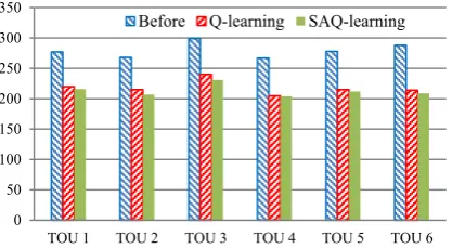
Figure 15 Economic cost comparison under different TOU mechanism

To illustrate the adaptability of the proposed method, we perform experiments under different TOU to test the economic reduction. The results of these tests are shown in Figure 15. The price of TOU1-TOU6 and their respective data sources are listed in Appendix A. As economic dispatch has a strong correlation with the load demand and price in each period, reduction of economic cost varies with different TOU mechanisms, but the differences are all obvious.

5. Conclusions

In this work, a dispatch optimization problem for a grid-connected MG with multi-objective is studied. Considering the reduction of economic cost and load rate cost, a dispatch optimization method by the control of multiple DESDs is introduced. First, we presented an MG model that includes the physical and stochastic characteristic of each unit inside. Second, we formulate the problem as a FHMDP model. Finally, a SAQ optimization method is adopted to solve the problem online. In this method, the optimal action under each state can be obtained by the state-action value, and those state-action pairs are used to form an optimal policy.

In this paper, we consider the control of active power flow and assume that the power factor of DTs is constant in each period. More realistically, we can consider the case that the reactive power flow is scheduled by the static var compensators (SVCs) or capacitor banks (CBs), and time-delay phenomena are considered. These two topics are interesting for further work. Other future work includes considering using neural networks (e.g., BP and RBF) to approximate the compact Q-factors, which are maintained in a list in this paper.

Acknowledgments: This work is financially supported by National Natural Science Foundation of China (61573126, 71231004), Program for New Century Excellent Talents in University (NCET-11-0626), and Research Fund for the Doctoral Program of Higher Education (20130111110007).

0 50 100 150 200 250 300 350

TOU 1 TOU 2 TOU 3 TOU 4 TOU 5 TOU 6

18 of 20

Author Contributions: Kai Lv planned the whole paper and contributed to paper drafting. Hao Tang contributed to the model selection and suggested on the methodology. Yijing Li and Xin Li provided guidance and key suggestions.

Conflicts of Interest: The authors declare no conflict of interest.

Appendix A：Several TOU price mechanisms

Durati on 0:00 ~ 1:00 1:00 ~ 2:00 2:00 ~ 3:00 3:00 ~ 4:00 4:00 ~ 5:00 5:00 ~ 6:00 6:00 ~ 7:00 7:00 ~ 8:00 8:00 ~ 9:00 9:00 ~ 10:00 10:00 ~ 11:00 11:00 ~ 12:00 TOU1(

$) 0.083 0.083 0.083 0.083 0.083 0.083 0.083 0.175 0.175 0.175 0.175 0.128

TOU

2($) 0.083 0.083 0.083 0.083 0.083 0.083 0.083 0.128 0.128 0.128 0.128 0.175

TOU

3($) 0.021 0.021 0.021 0.021 0.021 0.021 0.021 0.076 0.076 0.167 0.167 0.167

TOU

4($) 0.111 0.111 0.111 0.090 0.090 0.090 0.090 0.090 0.111 0.111 0.128 0.152

TOU

5($) 0.065 0.065 0.065 0.065 0.065 0.065 0.065 0.166 0.166 0.166 0.166 0.114

TOU

6($) 0.118 0.118 0.118 0.118 0.118 0.118 0.118 0.118 0.132 0.132 0.132 0.132

Durati on 12:00 ~ 13:00 13:00 ~ 14:00 14:00 ~ 15:00 15:00 ~ 16:00 16:00 ~ 17:00 17:00 ~ 18:00 18:00 ~ 19:00 19:00 ~ 20:00 20:00 ~ 21:00 21:00 ~ 22:00 22:00 ~ 23:00 23:00 ~ 24:00 TOU

1($) 0.128 0.128 0.128 0.128 0.128 0.175 0.175 0.083 0.083 0.083 0.083 0.083

TOU

2($) 0.175 0.175 0.175 0.175 0.175 0.128 0.128 0.083 0.083 0.083 0.083 0.083

TOU

3($) 0.167 0.167 0.167 0.167 0.167 0.167 0.167 0.167 0.167 0.167 0.167 0.167

TOU

4($) 0.152 0.152 0.111 0.111 0.128 0.128 0.128 0.128 0.128 0.128 0.128 0.111

TOU

5($) 0.114 0.114 0.114 0.114 0.114 0.114 0.114 0.166 0.166 0.166 0.166 0.065

TOU

6($) 0.132 0.132 0.132 0.132 0.132 0.132 0.132 0.132 0.132 0.118 0.118 0.118

References

[1] Hartono, B.S.; Budiyanto, Y.; Setiabudy R.. Review of microgrid technology. In proceedings of

International Conference on QiR(Quality in Research), Yogyakarta, The Republic of Indonesia,

25-28 June 2013; pp. 127 - 132

[2] Nguyen T; Crow M. Stochastic optimization of renewable-based microgrid operation

incorporating battery operating cost. IEEE Trans. Power Syst, 2015, 99, 1-8.

[3] Shi Q, Geng G, Jiang Q. Real-time optimal energy dispatch of standalone MG. Proceedings of

the Csee, 2012, 32, 26-35.

[4] Ayyanar R; Mohan N. A novel full-bridge DC-DC converter for battery charging using

secondary-side control combines soft-switching over the full load range and low magnetics

requirement. IEEE Trans. Ind. Electron., 2001, 37, 559-565.

[5] Elmakis D; Braunstein A; Naot Y. A probabilistic method for establishing the transformer

19 of 20

1988, 3, 920-925.

[6] Yu Y; Luan W. Smart grid and its implementations. Proceedings of the Csee, 2009, 29, 1-8.

[7] Puterman M.L.. Markov decision processes: discrete stochastic dynamic programming, 1st ed.; wiley

interscience: New Jersey, USA, 1994; pp. 74-118.

[8] DP Bertsekas. Dynamic programming and optimal control, 1st ed. Athena Scientific: Nashua, USA,

2000; pp. 94-114.

[9] Lattimore T; Hutter M; Sunehag P. The sample-complexity of general reinforcement learning.

In Proceedings of the International Conference on Machine Learning, Atlanta, USA, 16-21 June, 2013.

[10] Celebi E; Fuller JD. Time-of-Use pricing in electricity markets under different market structures.

IEEE Trans. Power Syst, 2012, 27, 1170-1181.

[11] Kirschen DS. Demand-side view of electricity markets. IEEE Trans. Power Syst, 2003, 2, 520-527.

[12] Mahmoodi M; Shamsi P; Fahimi B. Optimal scheduling of microgrid operation considering the

time-of-use price of electricity. In the Proceedings of the Conference of the IEEE Industrial Electronics Society, Vienna, Austria, 10-13 Nov. 2013.

[13] Du H; Liu S; Kong Q; Zhao W. A microgrid energy management system with demand response.

In Proceedings of China International Conference on Electricity Distribution, Shenzhen, China, 23-26 September, 2014; pp.2127 – 2132.

[14] Santis E.D.; Rizzi A; Sadeghiany A; Mascioli F.M.F.. Genetic Optimization of a Fuzzy Control

System for Energy Flow Management in MGs. In the Proceedings of Joint IFSA World

Congress and NAFIPS Annual Meeting, Edmonton, Canada, 24-28 June 2013; pp. 418-423.

[15] Liu H; Ji Y; Zhuang H; Wu H. Multi-objective dynamic economic dispatch of microgrid

systems including vehicle-to-grid. Energies, 2015, 8, 4476-4495.

[16] Rekik M; Abdelkafi A; Krichen L. A micro-grid ensuring multi-objective control strategy of a

power electrical system for quality improvement. Energy, 2015, 88, 351–363.

[17] Ahmadi A; Moghimi H; Nezhad A.E.; Agelidis V.G.; Sharaf A.M.. Multi-objective economic

emission dispatch considering combined heat and power by normal boundary intersection

method. Electric Power Systems Research, 2015, 129, 32-43.

[18] Zhong Y; Huang M; YE C. Multi-objective optimization of microgrid operation based on

dynamic dispatch of battery energy storage system. Electric Power Automation Equipment, 2014,

34, 113-121.

[19] Li C; Zhang J; Peng L. Multi-objective optimization model of MG operation considering cost,

pollution discharge and risk. Proceedings of the Csee, 2015, 35, 1051-1058.

[20] Miao Y; Jiang Q; Cao Y. Optimal microgrid dispatch considering stochastic integration of

electric vehicles. Electric Power Automation Equipment, 2013, 33, 1-7.

[21] Abido M. Environmental/economic power dispatch using multi-objective evolutionary

algorithms: a comparative study. IEEE Trans. Power Syst, 2003, 18, 920-925.

[22] Li F; Wu M; He Y; Chen X. Optimal control in microgrid using multi-agent reinforcement

learning. Isa Transactions, 2012, 51, 743-751.

[23] Harley R; Ben-Dov E. Lifetime estimation and monitoring of power transformer considering

annual load factors. IEEE Trans. Dielectrics & Electrical Insulation, 2014, 21, 1360-1367.

[24] Biçen Y; Aras F; Kirkici H. Optimal rating of a transformer for a growing load diagram. IEEE

20 of 20

[25] Huang Q; Jia Q; Guan X. Multi-timescale optimization between distributed wind generators

and electric vehicles in microgrid. In the Proceedings of the IEEE International Conference on Automation Science & Engineering, Goteborg, Sweden, 24-28 August 2015.

[26] Strrelec M; Berka J. Microgrid energy management based on approximate dynamic

programming. Innovative Smart Grid Technologies Europe, 2013, 2, 1-5.

[27] Tang H; Xu L; Sun J; Chen Y; Zhou L. Modeling and optimization control of a demand-driven,

conveyor-serviced production station. European Journal of Operational Research, 2015, 243,

839-851.

[28] Labeeuw W; Deconinck G. Residential electrical load model based on mixture model clustering

and markov models. IEEE Trans. Ind. Informat, 2013, 9, 1561-1569.

[29] Jardini J; Tahan C; Gouvea M; Ahn S. Daily load profiles for residential, commercial and

industrial low voltage consumers. IEEE Trans. Power Del, 2000, 15, 375-380.

[30] Bennett C; Stewart R; Lu J; Bennett C; Lu J. Autoregressive with exogenous variables and

neural network short-term load forecast models for residential low voltage distribution

networks. Energies, 2014, 7, 2938-2960.

[31] Marwali M; Haili M; Shahidehpour S; Abdul-Rahman K. Short term generation scheduling in

photovoltaic-utility grid with battery storage. IEEE Trans. Power Syst, 1998, 13, 1057-1062.

[32] Augugliaro A; Dusonchet L; SanseverinoE.R.. Voltage drop and power losses fast evaluation

through equivalent models of feeders for optimal operation of automated distribution

networks. European Transactions on Electrical Power, 1999, 9, 217–225.

[33] Paatero J; Lund P. A model for generating household electricity load profiles. International

Journal of Energy Research, 2006, 30, 273–290.

[34] Guo L; Liu W; Jiao B; Hong B. Multi-objective stochastic optimal planning method for

stand-alone microgrid system. Iet Generation Transmission & Distribution, 2014, 8, 1263-1273.

[35] Barnes A; Balda J; Rodriguez L. Complexity analysis and verification of real-time operation for

a semi-Markov model of photovoltaic intermittency. In Proceedings of the IEEE International Symposium on Power Electronics for Distributed Generation, 22-25 June 2015, Aachen, Germany.

[36] Barnes A; Balda J; Escobar-Mejia A. A semi-markov model for control of energy storage in

utility grids and microgrids with PV generation. IEEE Trans. Sustainable Energy, 2015, 6, 1-11.

[37]Giorgio A; Liberati F; Pietrabissa A. On-board stochastic control of electric vehicle recharging.

In Proceedings of the IEEE Conference on Decision and Control, 10-13 Dec 2013, Firenze, Italy. pp. 5710 – 5715.