Inverse Ramsey Problem of the Resource Misallocation Effect on Aggregate Productivity

Munich Personal RePEc Archive

Inverse Ramsey Problem of the Resource

Misallocation Effect on Aggregate

Productivity

Aoki, Shuhei

Graduate School of Economics, University of Tokyo

26 March 2008

Online at

https://mpra.ub.uni-muenchen.de/10973/

Inverse Ramsey Problem of the Resource

Misallocation Effect on Aggregate Productivity

Shuhei Aoki

Graduate School of Economics, University of Tokyo

October 7, 2008

Abstract

This paper examines the extent to and the conditions under which

re-source misallocation negatively affects aggregate productivity in a model

of heterogeneous firms to the highest degree. I analytically derive the

minimum aggregate total factor productivity (TFP) under resource

mis-allocation, when frictions are modeled as the taxes levied on a firm’s

output, and the range of these taxes is provided. I find that the lower

limit of the minimum aggregate TFP is the TFP under perfect substitute

goods and constant returns to scale technology. Further, with the

excep-tion of particular parameter values in which the misallocaexcep-tion effect on

aggregate TFP is small, the minimum aggregate TFP is achieved when

the proportion of firms in the lowest tax level is small or when the TFP

level of these firms is low.

Keywords: distortions; firm heterogeneity; misallocation; productivity;

Ramsey problem

JEL classification: O11, O41

∗_{Graduate School of Economics, University of Tokyo, 7-3-1, Hongo, Bunkyo-ku, Tokyo}

1

Introduction

Cross-country differences in the aggregate total factor productivity (TFP) are one of the important sources for the income disparity between developed and underdeveloped countries. A large body of research proposes mechanisms that explain the differences in the aggregate TFP. As Restuccia and Rogerson (2008) point out, many of these mechanisms can be characterized as the theory of resource misallocation. This theory states that frictions due to various reasons prevent the efficient use of resources, resulting in a low aggregate TFP.

This paper poses the following questions: To what extent do resource misal-locations affect the aggregate TFP? What kind of resource misallocation affects the aggregate TFP the most? This paper analytically addresses both these questions. There are two reasons for posing these questions. First, it is useful to know the applicability limit of the theory. Because there are infinite possibil-ities for resource misallocation between firms, the maximum effect of resource misallocation is not apparent. Second, the result provides information about the kind of resource misallocation mechanism researchers should focus on. While in the standard Ramsey problem, we analyze the conditions under which the maximum welfare is achieved, this paper analyzes the conditions under which the minimum aggregate TFP is achieved. In this sense, this paper inverses the standard Ramsey problem. Hence, I refer to this paper’s analysis as an inverse Ramsey problem.

In order to answer the abovementioned questions, I develop a simple model of monopolistic (or perfect) competition with heterogeneous firms that draws heavily from previous works (Melitz, 2003, Restuccia and Rogerson, 2008, Hsieh and Klenow, 2007, and Alfaro, Charlton and Kanczuk, 2008). Following Restuc-cia and Rogerson (2008), frictions are described as the taxes levied on a firm’s output. In this model, the differences in the taxes across firms result in resource misallocation and the loss of the aggregate TFP.1

1

Using the model, I address the abovementioned questions. I derive the min-imum level of this aggregate TFP when the lower and upper bounds of the tax levels are provided, and obtain the conditions under the minimum aggregate TFP.2 _{In the model, the higher the elasticity of substitution of goods and the}

firm’s returns to scale, the lower is the minimum aggregate TFP. The lower limit of the minimum aggregate TFP is the TFP under perfect substitute goods and constant returns to scale technology, where the minimum aggregate TFP relative to the TFP with no frictions is equal to the ratio of the gross maxi-mum and minimaxi-mum tax levels (the gross tax level implies 1−τ, where τ is the taxes levied on a firm’s output). The result suggests that researchers should focus on resource misallocation between firms or sectors that produce relatively substitutable goods.

Further, I find that with the exception of particular parameter values in which the effect of resource misallocation on the aggregate TFP is small, the minimum aggregate TFP is achieved if the proportion of firms in the minimum tax level is small or if the TFP of these firms is low. Thus, resource misallocation is not necessarily related to the TFP levels of firms.3 _{The result is consistent}

with the hypotheses that the aggregate TFP of underdeveloped countries is low because a small number of firms such as state-owned enterprises are protected by government policies or because the low TFP firms are protected by monopoly rights (Parente and Prescott, 1999) or by size-dependent policies (Guner, Ven-tura and Xu, 2008). However, this paper also reveals that to be consistent with data, the latter hypotheses might need some modifications, if goods are highly substitutive and the firm’s returns to scale is high. On the other hand, the re-sult suggests that the hypothesis that attributes the low aggregate TFP to the borrowing constraint of small firms might encounter difficulties when explaining

2

I select the ratio of the (gross) lower and upper tax levels as the basis of plausibility. Since the differences in the (gross) taxes imply the differences in the factor input returns, a large difference in the lower and upper tax levels is implausible from the viewpoint of arbitrage. Under the criterion, we need to explain the differences in the aggregate TFP with a reasonable ratio of these taxes. Parente and Prescott (2005, pp.1394–1395) developed a similar argument.

3

the low aggregate TFP in underdeveloped countries. Moreover, I find that we need to maintain caution when applying the lognormal approximation, which is widely used in the research.

There is a growing body of literature that analyzes the effect of resource misallocation on the aggregate TFP using the general equilibrium model of heterogeneous firms. Guner et al. (2008), Restuccia and Rogerson (2008), and Jones (2008) theoretically analyze the effect of resource misallocation under several scenarios. While their papers first consider the scenarios of resource misallocation and then analyze their effects on the aggregate TFP, this paper first determines the lowest level of the aggregate TFP resulting from resource misallocation and then analyzes the scenario that achieves the lowest aggregate TFP. Hsieh and Klenow (2007) and Alfaro et al. (2008), among others, measure frictions on resource misallocation and calculate the effect of these frictions on the aggregate TFP. This paper’s analysis will help analyze what kind of resource misallocation is important to their results.

The remainder of this paper is organized as follows. Section 2 introduces the model, and Section 3 defines the aggregate TFP. Given these settings, Section 4 solves the inverse Ramsey problem and analyzes the implication of the results. Finally, Section 5 presents the conclusions.

2

Model

2.1

Final goods sector

Firms in the final goods sector produce final goodsY from intermediate goods

{yi}. Further, firms in the final goods sector are competitive and maximize the

following problem:

max

{yi}

Y({yi})− ∫

piyidi,

where

Y({yi}) = (∫

y_iρdi

)1ρ

,

and pi is an intermediate good price. I assume thatρ≤1 and ρ̸= 0 (for the

lower bound ofρ, see the next section).

The first-order conditions (FOCs) are as follows:

pi=yiρ−1Y1−ρ, (1)

Y =

∫

piyidi. (2)

2.2

Intermediate goods sector

Firms in the intermediate goods sector produce intermediate goods yi from

capitalki and laborli. The profit maximization problem of a monopolistically

competitive intermediate goods firm is as follows: max

ki,li

(1−τi)piyi−rki−wli, (3)

s.t. yi=aikαil γ i,

where pi is given by (1), ai is the firm’s TFP, and r and w are the factor

costs of capital and labor, respectively. I assume that 0< α+γ ≤1 and that

ρ(α+γ)<1.

can instead consider a model in whichi corresponds to a sector and the firms in each sector are price takers. The results after Section 3 do not change even if we adopt the latter setting. When the intermediate firms are monopolistically competitive,ρhas to be more than zero. In Section 4, I also deal with the case where ρ < 0 because the ρ < 0 case is analyzed in some multi-sector models (e.g., Ngai and Pissarides, 2007 and Duarte and Restuccia, 2007). Thus, for the

ρ <0 case, I assume that the intermediate firms are perfectly competitive. From the FOCs, we obtain the following relation:

ki=

(1−τi)

r αρpiyi, (4)

li= 1

(1 +τli)w

γρpiyi.

2.3

Resource constraints

The following resource constraints are satisfied:

∫

kidi=K, ∫

lidi=L,

whereKandLare the aggregate supply of capital and labor, respectively, which are exogenously provided.

2.4

Equilibrium allocation

Here, I derive the equilibrium allocation ofY. Substituting (4) into the resource constraint of capital, we obtain

1

r =

K

∫

αρpiyiλidi

whereλi≡(1−τi). Substituting this equation into (4) and on rearranging, we

obtain

where ˜σi ≡ piyi/(∫ piyidi) and ˜λi ≡ λi/(∫ ˜σiλidi). In the same way, we can

obtain

li= ˜σiλ˜iL. (6)

By substituting the results arrived at,Y can be rewritten as follows:

Y =

[∫

aρi˜σ ρθ i ˜λ

ρθ i di

]1ρ

KαLγ,

whereθ≡α+γ.

In order to obtain the equilibrium allocation ofY, I derive the equilibrium allocations of ˜σi and ˜λi. Appendix A shows the following:

˜

σi=

aκρ_i λκρθ_i

W , (7)

whereκ≡1/(1−ρθ) and

W =

∫

aκρi λ κρθ

i di. (8)

Using (7), the denominator of ˜λi is written as follows: ∫

˜

σiλidi=

Z W,

where

Z=

∫

aκρi λκidi. (9)

Y as follows:4

Y = W

1

ρ

Zθ K

α_Lγ_{. (10)}

3

Aggregate TFP

I define the aggregate TFPA as follows:

A≡ Y

Kα_Lγ.

Subsequently, the aggregate TFP in equilibrium is given by

A=W

1

ρ

Zθ . (11)

This equation can be rewritten as follows:

A=A∗N,

where

A∗_≡ (∫

aκρ_di )1ρ−θ

,

N ≡

(∫ _aκρ i ∫

aκρi di

ν_iρdi

)1ρ/(∫ _aκρ i ∫

aκρi di

ν1θ

i di )θ

,

and νi ≡λκθi . A∗ is the aggregate TFP level when there is no friction. I refer

toN as the relative TFP because it corresponds to the aggregate TFP relative to the TFP with no frictions. Since

dHi≡ a

κρ i ∫

aκρ_i didi

4

can be considered as a distribution, N can be further revised as follows:

N =

(∫

ν_iρdHi

)ρ1/(∫

ν1θ

i dHi )θ

.

We can confirmN ≤1 from the property of power means, becauseρ <1/θ. In the following sections, I analyze howN can be lowered by resource mis-allocation. Moreover, I only consider the case wherein the number of tax levels is finite. Subsequently, N can be rewritten as follows (here, I slightly modify the notations):

N =

( ∑

i

hiνiρ

)1ρ/( ∑

i

hiν

1

θ

i )θ

,

wherehiis the proportion of firms in the same tax level, adjusted by the firm’s

TFP

hi≡ ∫

j:{νj=νi}

aκρj ∫

aκρj dj

dj. (12)

Obviously,∑

ihi= 1.

4

Inverse Ramsey Problem

4.1

Derivation of the minimum relative TFP

This section derives the minimum relative TFP,Nmin, when the gross minimum

tax level λs ≡ (1−τs) and the gross maximum tax level λt ≡ (1−τt) are

exogenously provided.5 _{Here, I use the subscript s for the variables with the}

minimum tax level, and subscript t for those with the maximum tax level. Obviously, we assume thatλs≥λt.

Owing to the following proposition, we only need to consider the distribution ofλsandλt(the proof is presented in Appendix B).

5

As will be revealed later, in fact, we do not need to determine the absolute values ofλs

Proposition 1. Nmin is achieved under the following condition: hs+ht= 1.

Then, the inverse Ramsey problem is as follows:

Nmin= min

hs

N (13)

s.t. N= (hsνsρ+htνtρ)

1

ρ

/ (

hsν

1

θ

s +htν

1

θ

t )θ

, (14)

hs+ht= 1.

From the FOC, we obtain hs, which achievesNmin,hs,minas follows:6

hs,min=

1 1−ρθ

( _ρθ

νρ₋₁−

1

ν1θ −1

)

,

where ν ≡νs/νt. By substituting this equation into (14), we obtain Nmin as

follows:

Nmin=

[ (_1−µ

1−ρθ

)1−ρθ(_µ

ρθ

)ρθ] 1

ρ

(15) where

µ≡ ν

ρ₋₁

ν1θ −1 = λ

ρθ

1−ρθ −1 λ1−1ρθ −1

, λ≡λs/λt.

Nmin has the following limit values:

Nmin−−−→

ρ→0 e

θ_λ− θ λ−1

(

lnλ λ−1

)θ

, (16)

−−−→

ρθ→1

1

λ. (17)

6

Appendix C proves that the second-order condition is positive (i.e., N obtained is the local minimum). Since N under the implicit corner solutions (hs = 0 andhs = 1) is equal

4.2

Analysis of the result

This section analyzes the results obtained in the previous section, when λ ≡

(1−τs)/(1−τt) is between one and ten.7

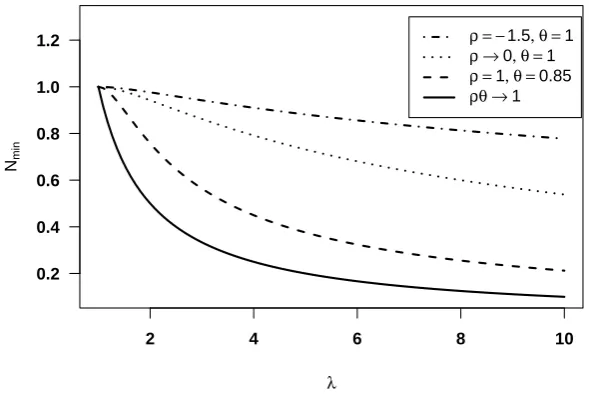
Figure 1 plots the minimum relative TFPNminfor the following three cases

using (15), (16), and (17): (i) ρ = −1.5 and θ = 1, (ii) ρ → 0 and θ = 1,

(iii) ρ = 1 andθ = 0.85, and (iv)ρθ → 1. The parameter values of the first case are similar to those used in Duarte and Restuccia (2007). The parameter values of the second case are similar to those in Restuccia, Yang and Zhu (2008) and Hayashi and Prescott (2008) in the long run.8 _{The third case corresponds}

to Restuccia and Rogerson (2008), and the fourth case corresponds to Parente and Prescott (1999). The second and third cases can generate a large loss of the aggregate TFP caused by resource misallocation, while the first case has a relatively low ability. One might infer from Figure 1 that Nmin lowers as ρθ

increases. This inference is correct (for an explanation, see Appendix D). The result is analogous to the implication of the standard Ramsey problem that taxes on goods with elastic demand highly distort welfare.

An interesting point is that the correlation of the firm’s TFP and tax level is not required to generate the above results. Although the firm’s TFP enters into hs, hs can be changed arbitrarily by changing the proportion of firms.

This result is particularly interesting when Nminconverges to the Parente and

Prescott (1999) case, because only at the limit, the proportion of firms does not affect the aggregate TFP.

Another interesting point is the discrepancy between the analysis in this paper and the lognormal approximation used in the literature.9 _{If we assume}

that the distribution of the firm’s TFP and tax is approximated by a joint lognormal distribution, from (11), the aggregate TFP can be approximated as

7

The value of ten forλcorresponds to, for example, the rental rate variation between 3% to 30% (under the same risk), which I think is reasonable as the upper bound.

8

The papers corresponding to the second to fourth cases pertain to the theory of resource misallocation.

9

follows (for the derivation, see Appendix E.1):

A≃exp

{

µlna+

1 2

1 1−ρθ

(

ρσ2lna−θσln2λ )

}

,

whereµlna is the mean of lnai, andσln2 aandσln2λ are the variances of lnai and

lnλi. Suppose thatσln2a = 0 andσln2λ>0. Then, asρθconverges to unity, the

aggregate TFP converges to zero, even if the variance of taxes is considerably small. The result stems from a characteristic of the lognormal distribution that its domain is unbounded. Our result suggests that caution is required when the lognormal approximation is applied.

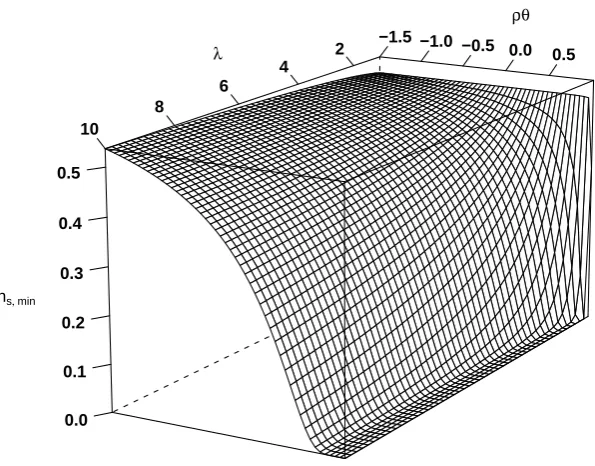
Next, I examine the composition of firms under the minimum relative TFP. I plot the hs under the minimum relative TFP, hs,min, in Figure 2. We find

that for small λ,hs,min is close to 0.5, regardless of the values of ρandθ. We

can verify the property by applying the second-order Taylor approximation to the logarithm of (14) aroundλ= 1 as follows (for the derivation, see Appendix E.2):

lnN ≃ −1

2

θ

1−ρθhs(1−hs)(λ−1)

2_.

Thus, forλaround unity,N(λ) becomes the minimum whenhs= 0.5.

On the other hand, hs,min becomes smaller as λ increases, except for the

caseρθ≤ −1. We can verify this as follows. When ρ >0, for sufficiently large

λ, N given by (14) approximately becomes as follows (for the derivation, see Appendix E.3):10

N ≃h1ρ−θ

s . (18)

Since 1/ρ−θ >0, thisN becomes smaller, ashs decreases. When ρ <0, for

sufficiently largeλ,N given by (14) approximately becomes as follows (for the

10

(18) also achieves the lower bound of Restuccia and Rogerson’s (2008) numerical exper-iment. For example, in their uncorrelated case, wherein the frictions were uncorrelated with the firm’s TFPs,hscorresponds to 0.5. Then, the lower bound of the relative TFP given by

(18) is (1/2)0.15

derivation, see Appendix E.4):

N = 1

h−ρ1

t hθsλ

θ

1−ρθ

. (19)

The result shows that when ρθ >−1, as in the case that ρ > 0, N becomes smaller as hs decreases. However, when ρθ ≤ −1, N becomes smaller as hs

increases.

Moreover, Figure 2 shows that hs,min decreases as ρθ increases. This is

because, as (18) and (19) suggest, the maximum effect of the frictions lowers as

ρθincreases. In order to compensate for it, hs should be lower.

4.3

What kind of resource misallocation should be focused

on?

The results in the previous section suggest that in order to understand the large differences in aggregate TFP between developed and underdeveloped countries, it is important to focus on resource misallocation between firms or sectors that produce relatively substitutable goods that corresponds to the ρ > 0 in our model.

It is also important to explore the resource misallocations that are consis-tent with small hs in order to consider the source of the large differences in

aggregate TFP. The hypothesis that a small proportion of firms, for example, state-owned enterprises, are selectively protected by the government policies is consistent with small hs. The hypothesis that low TFP firms are protected is

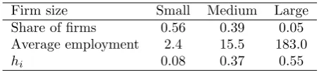
also consistent with small hs. Table 1 reports the hi of firms (referred to as

Roger-son (2008).11 _Theh

i of firms with the lowest TFP is 0.08, although such firms

constitute more than half of all firms. Hence, if firms with the lowest TFP are protected, it considerably lowers the aggregate TFP. However, it should also be noted that hs,min with high ρθ and relatively high λis smaller than 0.08, for

example, hs,min at ρθ= 0.85 andλ= 2 is less than 0.05 (see Figure 3, which

plots the limits ofρθabove whichhs,minfalls below 0.08). Thus, even if we focus

on resource misallocation with respect to the low TFP firms, it is important to explore the possibility that some of the low TFP firms are selectively protected. On the other hand, it might be difficult to explain the large differences in the aggregate TFP by means of the borrowing constraint of small firms. This is because these small firms belong to (1−hs,min) of firms, while as observed in

Table 1, the hi of small firms is marginal.

5

Conclusion

This paper analytically examines the extent to and the conditions under which resource misallocation negatively affects the aggregate TFP to the highest de-gree, when frictions are modeled as the taxes levied on a firm’s output. The implications derived from the analysis would be effective in researching the mechanisms of resource misallocation that explain the differences in the aggre-gate TFP of developed and underdeveloped countries.

There are several important issues that still need to be addressed in future research. First, while I derive the minimum aggregate TFP when the lower and upper tax levels are provided, other specifications on the constraint of frictions might be possible. Second, I abstract from fixed costs. Qualitatively, under

11

Using (12), thehiis measured as

hi=

giaκρi

∑

igiaκρi

=∑gili

igili

,

wheregiis the fraction ofifirms, andliis firmi’s labor input of the U.S. under the assumption

that the U.S. is an economy with no frictions. Note that the measuredhidoes not depend on

fixed costs, higher frictions on the lower TFP firms (higher frictions imply higher taxes in this paper’s model) can discourage these firms from operation and entry, which results in lowering the aggregate TFP. Thus, lower frictions on a small proportion of relatively high TFP firms negatively affect the aggregate TFP the most. In order to quantitatively analyze this effect, assumptions on the fixed costs and the distribution of firms that are not arbitrary are required. Finally, as emphasized in Jones (2008), the existence of material inputs could magnify the resource misallocation effect.

References

Alfaro, Laura, Andrew Charlton, and Fabio Kanczuk (2008) “Plant-Size Dis-tribution and Cross-Country Income Differences”, NBER Working Papers 14060, National Bureau of Economic Research, Inc.

Duarte, Margarida and Diego Restuccia (2007) “The Role of the Structural Transformation in Aggregate Productivity”, Working Papers tecipa-300, Uni-versity of Toronto, Department of Economics.

Guner, Nezih, Gustavo Ventura, and Yi Xu (2008) “Macroeconomic Implica-tions of Size-Dependent Policies”, Review of Economic Dynamics, Vol. 11, No. 4, pp. 721–744.

Hayashi, Fumio and Edward C. Prescott (2008) “The Depressing Effect of Agri-cultural Institutions on the Prewar Japanese Economy”,forthcoming in Jour-nal of Political Economy.

Hsieh, Chang-Tai and Peter J. Klenow (2007) “Misallocation and Manufacturing TFP in China and India”, NBER Working Papers 13290, National Bureau of Economic Research, Inc.

Manuelli, Rodolfo E. (2003) “Policy Uncertainty, Total Factor Productivity and Growth”. Mimeo.

Melitz, Marc J. (2003) “The Impact of Trade on Intra-Industry Reallocations and Aggregate Industry Productivity”, Econometrica, Vol. 71, No. 6, pp. 1695–1725.

Ngai, L. Rachel and Christopher A. Pissarides (2007) “Structural Change in a Multisector Model of Growth”, American Economic Review, Vol. 97, No. 1, pp. 429–443.

Parente, Stephen L. and Edward C. Prescott (1999) “Monopoly Rights: A Bar-rier to Riches”,American Economic Review, Vol. 89, No. 5, pp. 1216–1233.

(2005) “A Unified Theory of the Evolution of International Income Lev-els”, in Philippe Aghion and Steven Durlauf eds. Handbook of Economic Growth, Vol. 1 of Handbook of Economic Growth: Elsevier, Chap. 21, pp. 1371–1416.

Restuccia, Diego and Richard Rogerson (2008) “Policy Distortions and Aggre-gate Productivity with Heterogeneous Establishments”,Review of Economic Dynamics, Vol. 11, No. 4, pp. 707–720.

Appendix

A

Derivation of

σ

_˜

By using (1) and (2), ˜σi can be written as follows:

˜

σi=

y_iρ Yρ

= a

ρ iσ˜

ρθ i λ

ρθ i ∫

aρ_iσ˜_iρθλρθ_i di,

whereθ≡α+γ. By rewriting this equation, we obtain ˜

σi=

aκρi λ κρθ i

W ,

whereκ≡1/(1−ρθ) andW is defined as

W ≡

(∫

aρi˜σ ρθ i λ ρθ i di )κ .

W can be further extended as follows:

W =



 ∫

aρ_iλρθ_i

(

aκρ_i λκρθ_ii W )ρθ di   κ .

By rearrangingW, we thus obtain

W =

∫

aκρ_i λκρθ_i di.

Using this result, ˜σi can be expressed by exogenous variables.

B

Proof of Proposition 1

I prove Proposition 1 by contradiction.

Suppose that there arentax levels betweenλsandλtwith positivehi.

should be satisfied:

∂lnN ∂νi

= 0, for allνi betweenνsandνt.

If these conditions are not satisfied,N can be lowered by changingλi between

λsandλt. ∂lnN /∂νi is given by

∂lnN ∂νi

= hi

νi 

 

1

hi+∑m̸=ihm (

νm

νi

)ρ −

1

hi+∑_m̸=ihm (

νm

νi

)θ1





= 0. (20)

From this condition, we obtain

νρ−1θ

i =

∑

mhmνmρ

∑ mhmν

1

θ

m

.

Since this condition holds for anyνj betweenνsandνt,νi=νj. Thus, we only

need to consider the case wherein there is oneνi betweenνsandνt.

Next, I examine the second-order condition (SOC) of lnN when (20) is satisfied. I refer to the denominator of the first term in the parenthesis in (20) as B, and the second term asC. Then,

∂2_lnN

∂ν2

i

=−hi

ν2 i ( 1 B − 1 C )

+hi

νi (

ρ νi

B−hi

B2 −

1

θνi

C−hi

C2

)

= θhi

ν2 i hs ( νs νi )ρ

+ht (

νt

νi

)ρ

B2 (ρθ−1)≤0.

Equality holds only ifhs=ht= 0. Then, the maximum ofN is achieved.

Oth-erwise, N becomes the local maximum. Both cases contradict the assumption that N is the minimum.

C

Second-Order Condition of

N

I demonstrate that the SOC of the problem provided in (13) is positive for

The FOC is given by

∂lnN ∂hs

= 1

ρ b B −θ

c C = 0,

whereb≡νρ s−ν

ρ

t,B≡hsνsρ+htνtρ,c≡ν

1/θ

s −νt1/θ, andC≡hsνs1/θ+htνt1/θ.

The SOC when the FOC is satisfied is

∂2_lnN

∂h2

s

=−1

ρ

(

b B

)2

+θ(c C

)2

=θ(c C

)2

(1−ρθ)>0.

D

N

Lowers as

ρθ

→

1

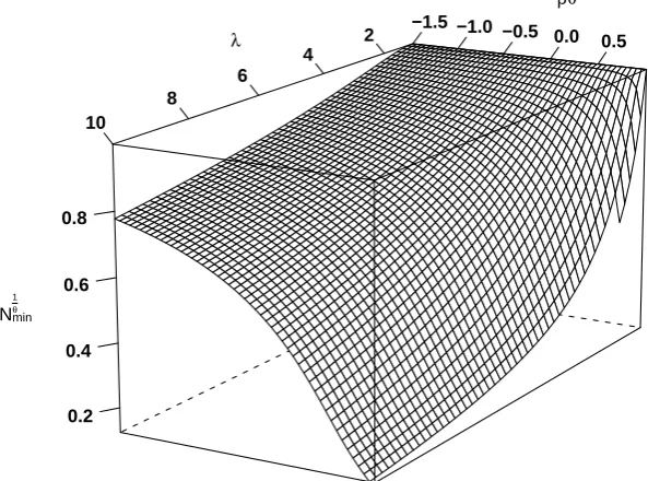
Figure 4 displays Nmin powered by 1/θ, over the ranges of ρθ and λ. In this

figure, for any λ, N_min1/θ lowers as ρθ increases. The shape of the figure is pre-served forNmin. Thus, for any givenθ,Nminalso lowers asρθ increases (i.e.,ρ

increases). In addition, for any givenρθ,Nminlowers asθincreases. Therefore,

Nmin lowers asρandθincrease.

E

Derivation of Approximations in Section 4.2

This appendix derives approximations employed in Section 4.2.

E.1

Lognormal approximation of

A

Suppose that xi is a variable of intermediate firm i. Then, the following

ap-proximation holds:

ln

(∫

xidi )

≃µlnx+

1 2σ

2 lnx,

where µlnx and σln2x are the mean and variance of lnxi. By applying this

we obtain lnW1ρ ≃κ

{

µlna+θµlnλ+

1 2

[

κρσ2lna+κρθ2σln2λ+ 2κρθσlna,lnλ] }

,

lnZθ≃κ

{

ρθµlna+θµlnλ+

1 2

[

κρ2θσln2a+κθσln2λ+ 2κρθσlna,lnλ ]

}

,

whereσlna,lnλis the covariance of lnai and lnλi. Therefore, from (11) and the

above approximations, we obtain lnA≃µlna+

1 2

1 1−ρθ

(

ρσln2a−θσ2lnλ )

.

E.2

ln

N

when

λ

is close to unity

Rewriting N in (14) using the definitions νi ≡ λiθ/(1−ρθ) and λ ≡ λs/λt, we

obtain

N(λ) =(hsλ ρθ

1−ρθ +h_t) 1

ρ (hsλ

1

1−ρθ +h_t)θ

. (21)

(Here, I explicitly writeN as the function ofλ.)

By applying the second-order Taylor expansion around λ = 1, lnN(λ) is approximately written as follows (here, for the simplicity of calculation, I take log to N):

lnN(λ)≃lnN(1) + lnN′(1)(λ−1) +lnN

′′₍₁₎

2 (λ−1)

2_.

Since lnN(1) = 0, lnN′_{(1) = 0, and lnN}′′_{(1) =−θ/(1−ρθ)h}

s(1−hs),

lnN(λ)≃ −1

2

θ

1−ρθhs(1−hs)(λ−1)

2_,

E.3

N

when

λ

is large: the

ρ >

0

case

Whenλis large andρ >0, from (21), we obtain

N(λ)≃(hsλ

ρθ

1−ρθ) 1

ρ (hsλ

1 1−ρθ)θ

=h1ρ−θ

s .

E.4

N

when

λ

is large: the

ρ <

0

case

Defineη ≡ −ρ >0. Then, from (21), we obtain

N(λ) = λ

θ

1−ρθ

(

hs+htλ

ηθ

1−ρθ

)1η(

hsλ

1 1−ρθ +h_t

)θ

≃ λ

θ

1−ρθ h1η

thθsλ

2θ

1−ρθ

= 1

h1η

thθsλ

θ

1−ρθ .

From the first line to the second line, I apply an approximation assuming that

Firm size Small Medium Large Share of firms 0.56 0.39 0.05 Average employment 2.4 15.5 183.0

hi 0.08 0.37 0.55

Table 1: Distribution of firms. Notes: These numbers were obtained and cal-culated from Table 2 of Restuccia and Rogerson (2008) (firms are referred to as establishments in their paper). hi is the proportion of firms with the same

TFP level, adjusted by their TFP, and is calculated in a manner similar to (12) (here, hi is for firms with the same TFP level instead of the same tax level).

2 4 6 8 10 0.2

0.4 0.6 0.8 1.0 1.2

λ Nm

in

ρ = −1.5, θ =1 ρ →0, θ =1 ρ =1, θ =0.85 ρθ →1

Figure 1: The minimum relative TFP, Nmin, under different parameter values.

2 4 6 8 10

−1.5 −1.0 −0.5 _0.0 0.5

0.0 0.1 0.2 0.3 0.4 0.5

λ

ρθ

hs, min

Figure 2: Proportion of firms with the lowest tax level, adjusted by the firm’s TFP,hs,minthat generates the minimum relative TFP, Nmin, under a range of

parameter values. Notes: ρis the parameter on the substitutability of goods. θ

is the firm’s returns to scale. λis the ratio of the gross lowest and highest tax levels, (1−τs)/(1−τt).

2 4 6 8 10

0.6 0.7 0.8 0.9 1.0

λ

ρθ

Figure 3: The limit of ρθ above which hs,min that generates Nmin falls below

0.08, for each λ. Notes: ρis the parameter on the substitutability of goods. θ

is the firm’s returns to scale. λis the ratio of the gross lowest and highest tax levels, (1−τs)/(1−τt). For example, for λ= 2,ρθ≈0.82, which implies that

2 4 6 8 10

−1.5 −1.0 −0.5 _0.0 0.5

0.2 0.4 0.6 0.8

λ

ρθ

Nmin

1 θ

Figure 4: The minimum relative TFP powered by 1/θ,N_min1/θ under a range of parameter values. Notes: ρis the parameter on the substitutability of goods.