Feature Selection for Intrusion Detection Using Random Forest

http://dx.doi.org/10.4236/jis.2016.73009

Feature Selection for Intrusion Detection

Using Random Forest

Md. Al Mehedi Hasan, Mohammed Nasser, Shamim Ahmad, Khademul Islam Molla

Department of Computer Science & Engineering, University of Rajshahi, Rajshahi, Bangladesh

Received 11 September 2015; accepted 4 April 2016; published 7 April 2016

Copyright © 2016 by authors and Scientific Research Publishing Inc.

This work is licensed under the Creative Commons Attribution International License (CC BY). http://creativecommons.org/licenses/by/4.0/

Abstract

An intrusion detection system collects and analyzes information from different areas within a computer or a network to identify possible security threats that include threats from both outside as well as inside of the organization. It deals with large amount of data, which contains various ir-relevant and redundant features and results in increased processing time and low detection rate. Therefore, feature selection should be treated as an indispensable pre-processing step to improve the overall system performance significantly while mining on huge datasets. In this context, in this paper, we focus on a two-step approach of feature selection based on Random Forest. The first step selects the features with higher variable importance score and guides the initialization of search process for the second step whose outputs the final feature subset for classification and in-terpretation. The effectiveness of this algorithm is demonstrated on KDD’99 intrusion detection datasets, which are based on DARPA 98 dataset, provides labeled data for researchers working in the field of intrusion detection. The important deficiency in the KDD’99 data set is the huge num- ber of redundant records as observed earlier. Therefore, we have derived a data set RRE-KDD by eliminating redundant record from KDD’99 train and test dataset, so the classifiers and feature selection method will not be biased towards more frequent records. This RRE-KDD consists of both KDD99Train+ and KDD99Test+ dataset for training and testing purposes, respectively. The experimental results show that the Random Forest based proposed approach can select most im-portant and relevant features useful for classification, which, in turn, reduces not only the number of input features and time but also increases the classification accuracy.

Keywords

1. Introduction

The internet and local area networks are growing larger in recent years. As a great variety of people all over the world are connecting to the Internet, they are unconsciously encountering the number of security threats such as viruses, worms and attacks from hackers [1]. Now firewalls, anti-virus software, message encryption, secured network protocols, password protection and so on are not sufficient to assure the security in computer networks, when some intrusions take advantages of weaknesses in computer systems to threaten. Therefore, Intrusion De-tection Systems (IDSs) have become a necessary addition to the security infrastructure of most organizations

[2].

Deploying highly effective IDS systems is extremely challenging and has emerged as a significant field of re-search, because it is not theoretically possible to set up a system with no vulnerabilities [3]. Several machine learning (ML) algorithms, for instance Neural Network [4], Genetic Algorithm [5], Support Vector Machine [2] [6], Clustering Algorithm [7] and more have been extensively employed to detect intrusion activities from large quantity of complex and dynamic datasets.

Current Intrusion Detection Systems (IDS) examine all data features to detect intrusion or misuse patterns [8]. Since the amount of audit data that an IDS needs to examine is very large even for a small network, therefore their analysis is difficult even with computer assistance because extraneous features can make it harder to detect suspicious behavior patterns [8]-[10]. As a result, IDS must reduce the amount of data to be processed. This is very important if a real-time detection is desired. Reduction can be performed by data filtering, data clustering or feature selection. In our work, we investigate feature selection to reduce the amount of data directly handled by the IDS.

Literature survey showed that, most of the researchers used randomly generated records or a portion of record from the KDD’99 dataset to develop feature selection method and to build intrusion detection system [1][8][10] [11] without using the whole train and test dataset. Yuehui Chen et al. [8], Srilatha et al. [10][11] present a re-duced number of features by using a randomly generated dataset containing only 11,982 records [8][10][11], therefore, the number of features reduced to 12 or 17 [10][11] is in question if the property of whole dataset is considered. So, those findings do not indicate the actual relevant features for classification. Although some re-searcher use the whole dataset but do not remove redundant records, which implies a limitation of having a chance of redundant record used for the same feature selection and because of that, classification methods may be biased toward to the class that has redundant records [12]. These limitations have motivated us to find out the actual relevant features for classification based on the whole train and test dataset of KDD’99 by removing re-dundant record.

Feature selection also known as variable selection, feature reduction, attribute selection or variable subset se-lection, is a widely used dimensionality reduction technique, which has been the focus of much research in ma-chine learning and data mining and has found applications in text classification, web mining, and so on [1]. It allows faster model building by reducing the number of features, and also helps removing irrelevant, redundant and noisy features. This begets simpler and more comprehensible classification models with classification per-formance. Hence, selecting relevant attributes are a critical issue for competitive classifiers and for data reduc-tion. Feature Selection can fall into two approaches: filter and wrapper [13]. The difference between the filter model and wrapper model is whether feature selection relies on any learning algorithm. The filter model is in-dependent of any learning algorithm, and its advantages lies in better generality and low computational cost [13]. It ranks the features by a metric and eliminates all features that do not achieve an adequate score (selecting only important features). The wrapper model relies on some learning algorithm, and it can expect high classification performance, but it is computationally expensive especially when dealing with large scale data sets [14] like KDDCUP99. It searches for the set of possible features for the optimal subset. In this paper, we adapt Random Forest to rank the features and select a subset feature, which can bring to a successful conclusion of intrusion detection.

Random Forest directly performs feature selection while a classification rule is built. The two commonly used variable importance measures in RF are Gini importance index and permutation importance index (PIM) [15]. In this paper, we have used two steps approach to feature selection. In first step, permutation importance index are used to rank the features and then in second step, Random Forest is used to select the best subset of features for classification. This reduced feature set is then employed to implement an Intrusion Detection System. Our ap-proach results in more accurate detection as well as fast training and testing process.

outline mathematical overview of RF and calculation procedure of variable importance in Section 3. Experi-mental setup is presented in Section 4 and RF model selection is drawn in Section 5. Measurement of Variable Importance and Variable Selection are discussed in section 6. Finally, Section 7 reports the experimental result followed by conclusion in Section 8.

2. KDDCUP’99 Dataset

Under the sponsorship of Defense Advanced Research Projects Agency (DARPA) and Air Force Research La-boratory (AFRL), MIT Lincoln LaLa-boratory has collected and distributed the datasets for the evaluation of re-searches in computer network intrusion detection systems [16]. The KDD’99 dataset is a subset of the DARPA benchmark dataset prepared by Sal Stofo and Wenke Lee [17]. The KDD data set was acquired from raw tcpdump data for a length of nine weeks. It is made up of a large number of network traffic activities that in-clude both normal and malicious connections.

2.1. Attack and Feature Description of KDD’99 Dataset

The KDD’99 data set includes three independent sets; “whole KDD”, “10% KDD”, and “corrected KDD”. Most of researchers have used the “10% KDD” and the “corrected KDD” as training and testing set, respectively [18]. The training set contains a total of 22 training attack types and one type for normal. The “corrected KDD” test-ing set includes an additional 17 types of attack and excludes 2 types (spy, warezclient) of attack from traintest-ing set, so therefore there are 37 attack types that are included in the testing set, as shown in Table 1 and Table 2. The simulated attacks fall in one of the four categories [2][18]: 1) Denial of Service Attack (DoS), 2) User to Root Attack (U2R), 3) Remote to Local Attack (R2L), 4) Probing Attack.

A connection in the KDD’99 dataset is represented by 41 features, each of which is in one of the continuous, discrete and symbolic forms, with significantly varying ranges [19] (Table 3). The description of various fea-tures is shown in Table 3. In Table 3, C is used to denote continuous and D is used to donate discrete and sym-bolic type data in the Data Type field.

2.2. Inherent Problems and Criticisms against the KDD’99

Statistical analysis on KDD’99 dataset found important issues which highly affects the performance of evaluated systems and results in a very poor evaluation of anomaly detection approaches [20]. The most important defi-ciency in the KDD data set is the huge number of redundant records. Analyzing KDD train and test sets, Moh-bod Tavallaee found that about 78% and 75% of the records are duplicated in the train and test set, respectively

[21]. This large amount of redundant records in the train set will cause learning algorithms to be biased towards the more frequent records.

As a result, this biasing prevents the system from learning infrequent records which are usually more harmful

Table 1. Attacks in KDD’99 training dataset.

Classification of Attacks Attack Name

Probing Port-sweep, IP-sweep, Nmap, Satan

DoS Neptune, Smurf, Pod, Teardrop, Land, Back

U2R Buffer-overflow, Load-module, Perl, Rootkit

R2L Guess-password, Ftp-write, Imap, Phf, Multihop, Spy, Warezclient, Warezmaster

Table 2. Attacks in KDD’99 testing dataset.

Classification of Attacks Attack Name

Probing Port-sweep, IP-sweep, Nmap, Satan, Saint, Mscan

DoS Neptune, Smurf, Pod, Teardrop, Land, Back, Apache2,Udpstorm, Processtable, Mail-bomb

U2R Buffer-overflow, Load-module, Perl, Rootkit, Xterm, Ps, Sqlattack.

Table 3. List of Features with their descriptions and data types.

S.

No Feature Description

Data Type

S.

No Feature Description

Data Type

1 Duration Duration of the

connection. C 22 Is guest login

1 if the login is a “guest” login; 0

otherwise D

2 Protocol type Connection protocol D 23 Count

Number of connections to the same host as the current connection in the past two seconds

C

3 Service Destination service D 24 Srv count

Number of connections to the same service as the current connection in the past two seconds

C

4 Flag Status flag of the

connection D 25 Serror rate

% of connections that have “SYN”

errors C

5 Source bytes Bytes sent from source

to destination C 26 Srv serror rate

% of connections that have “SYN”

errors C

6 Destination bytes Bytes sent from

destination to source C 27 Rerror rate

% of connections that have “REJ”

errors C

7 Land

1 if connection is from/to the same host/port; 0 otherwise

D 28 Srv rerror rate % of connections that have “REJ”

errors C

8 Wrong fragment Number of wrong

fragments C 29 Same srv rate % of connections to the same service C

9 Urgent Number of urgent

packets C 30 Diff srv rate

% of connections to different Services

C

10 Hot Number of “hot”

indicators C 31 Srv diff host rate % of connections to different hosts C

11 Failed Login Logins number of failed

logins C 32

Dst host count Count of connections having the same destination host

C

12 Logged in 1 if successfully logged

in; 0 otherwise D 33

Dst host srv count Count of connections having the same destination host and using the same service

C

13 Compromised

Number of “compromised” conditions

C 34 Dst host same srv rate

% of connections having the same destination host and using the same service

C

14 Root shell 1 if root shell is

obtained; 0 otherwise C 35 Dst host diff srv rate

% of different services on the current

host C

15 Su attempted 1 if “su root” command

attempted; 0 otherwise C 36

Dst host same src port rate

% of connections to the current host having the same src port

C

16 Root Number of “root”

accesses C 37

Dst host srv diff host rate

% of connections to the same service coming from different hosts

C

17 File creations Number of file creation

operations C 38 Dst host serror rate

% of connections to the current host that have an S0 error

C

18 Shells Number of shell

prompts C 39

Dst host srv serror rate

% of connections to the current host and specified service that have an S0 error

C

19 Access files Number of operations _{on access control files} C 40 Dst host rerror rate % of connections to the current host _{that have an RST error} C

20 Outbound cmds

Number of outbound commands in an ftp session

C 41 Dst host srv rerror _rate

% of connections to the current host and specified service that have an RST error

C

21 Is hot login

1 if the login belongs to the “hot” list; 0 otherwise

to networks such as U2R attacks. The existence of these repeated records in the test set, on the other hand, will cause the evaluation results to be biased by the methods which have better detection rates on the frequent records.

To solve these issues, we have derived a new data set RRE-KDD by eliminating redundant record from KDD’99 train and test dataset (10% KDD and corrected KDD), so the classifiers will not be biased towards more frequent records. This RRE-KDD dataset consists of KDD99Train+ and KDD99Test+ dataset for training and testing purposes, respectively. The numbers of records in the train and test sets are now reasonable, which makes it affordable to run the experiments on the complete set without the need to randomly select a small por-tion.

3. Variable Selection and Classification

Consider the problem of separating the set of training vectors belong to two separate classes, (x1, y1), (x2, y2), …, (xn, yn) where pand

{

}

i i

x ∈R y ∈ −， is the corresponding class label, 1 ≤ i ≤ n. The main task is to find a classifier with a decision function f(x, θ) such that y = f(x, θ), where y is the class label for x, θ is a vector of un-known parameters in the function.

3.1. Random Forest

The random forest is an ensemble of unpruned classification or regression trees [15]. Random forest generates many classification trees and each tree is constructed by a different bootstrap sample from the original data us-ing a tree classification algorithm. After the forest is formed, a new object that needs to be classified is put down each of the tree in the forest for classification. Each tree gives a vote that indicates the tree’s decision about the class of the object. The forest chooses the class with the most votes for the object. The random forests algorithm (for both classification and regression) is as follows [22][23]:

1) From the Training of n samples draw ntree bootstrap samples.

2) For each of the bootstrap samples, grow classification or regression tree with the following modification: at each node, rather than choosing the best split among all predictors, randomly sample mtry of the predic-tors and choose the best split among those variables. The tree is grown to the maximum size and not pruned back. Bagging can be thought of as the special case of random forests obtained when mtry = p, the number of predictors.

3) Predict new data by aggregating the predictions of the ntree trees (i.e., majority votes for classification, av-erage for regression).

There are two ways to evaluate the error rate. One is to split the dataset into training part and test part. We can employ the training part to build the forest, and then use the test part to calculate the error rate. Another way is to use the Out-of-Bag (OOB) error estimate. Because random forests algorithm calculates the OOB error during the training phase, therefore to get OOB error, we do not need to split the training data. In our work, we have used both ways to evaluate the error rate.

There are three tuning parameters of Random Forest: number of trees (ntree), number of descriptors randomly sampled as candidates for splitting at each node (mtry) and minimum node size [23]. When the forest is growing, random features are selected at random out of the all features in the training data. The number of features em-ployed in splitting each node for each tree is the primary tuning parameter (mtry). To improve the performance of random forests, this parameter should be optimized. The number of trees should only be chosen to be sufficient-ly large so that the OOB error has stabilized. In many cases, 500 trees are sufficient (more are needed if de-scriptor’s importance or intrinsic proximity is desired). In contrast to other algorithms having a stopping rule, in RF, there is no penalty for having “too many” trees, other than waste in computational resources. Another para-meter, minimum node size, determines the minimum size of nodes below which no split will be attempted. This parameter has some effect on the size of the trees grown. In Random Forest, for classification, the default value of minimum node size is 1, ensuring that trees are grown to their maximum size and for regression, the default value is 5 [23].

3.2. Variable Important Measure and Selection Using Random Forest

avoid over fitting and improve model performance, and 2) to gain a deeper insight into the underlying processes that generated the data [24]. The interpretability of machine learning models is treated as important as the pre-diction accuracy for most life science problems.

Unlike most other classifiers, Random Forest directly performs feature selection while a classification rule is built [25]. The two commonly used variable important measures in RF are Gini importance index and permuta-tion importance index (PIM) [15]. Gini importance index is directly derived from the Gini index when it is used as a node impurity measure. A feature’s importance value in a single tree is the sum of the Gini index reduction over all nodes in which the specific feature is used to split. The overall variable importance for a feature in the forest is defined as the summation or the average of its importance value among all trees in the forest. Permuta-tion importance measure (PIM) is arguably the most popular variable’s importance measure used in RF. The RF algorithm does not use all training samples in the construction of an individual tree. That leaves a set of out of bag (OOB) samples, which can be used to measure the forest’s classification accuracy. In order to measure a specific feature’s importance in the tree, randomly shuffle the values of this feature in the OOB samples and compare the classification accuracy between the intact OOB samples and the OOB samples with the particular feature permutated. In this work, we have used permutation importance measure (PIM) and developed two algo-rithms to measure PIM and select an important subset of feature among all features, as shown in Algorithm 1 and Algorithm 2.

Algorithm 1 (Step One): Measure of Variable Importance

1) Build 50 Random Forest. For each Random Forest, k = 1 to 50, repeat Steps 2 to 4. 2) For each tree t of the k-th Random Forest, Consider the associated OOBt sample. 3) Denoted by errOOB_t the error of a single tree t on this OOBt sample.

4) Randomly permute the values of Xj in OOBt to get a perturbed sample denoted by OOBtj After that,

compute errOOB_t and the difference of the error between the intact OOB samples and the OOB sam-ples with the permutated feature Xj. Finally, find out permutation importance measure (PIM) for the per-muted feature Xj using the following equation:

( )

(

)

tree

1

OOB OOB

j j

k t t

t

PIM X err err

n

=

∑

5) Find out the average permutation importance measure (APIM) of each variables from the 50 Random Forest using following equation

( )

( )

1

1 50

j j

k k

APIM X PIM X

= =

∑

Algorithm 2 (Step Two): Variable Selection:

1) Rank the variables by sorting the APIM score (averaged from the 50 runs of RF using Algorithm 1) in descending order.

2) Perform a sequential variable introduction with testing: a variable is added only if the error gain exceeds a threshold. The variables of the last model are selected.

4. Dataset and Experimental Setup

To select the best model in model selection phase, we have drawn 10% samples from the training set (KDDTrain+) to tune the parameters of all kernel and another 10% samples from the training set (KDDTrain+) to validate those parameters, as shown in Table 4.

5. Model Selection of RF

In order to generate highly performing classifiers capable of dealing with real data an efficient model selection is required. In this section, we present the experiments conducted to find efficient model for RF. To improve the detection rate, we optimize the number of the random features (mtry) which is used to build the RF. We build the forest with different mtry (5, 6, 7, 10, 15, 20, 25, 30, 35, and 38) over the train set (TrainSet) with keeping ntree = 100, then plot the OOB error rate and the time required to build the classifier RF versus different values of mtry. As Figure 1 shows, the OOB error rate reaches its minimum when the value of mtry is 7. Besides this, it is ob-vious that increasing in mtry increases the time required to build the classifier. Thus, we choose the value of mtry = 7 as the optimal value, which reaches at the minimum value of the OOB error rate and does cost moderately the least time among these values.

There are two other parameters in Random Forest: number of trees and minimum node size. In order to find out the value of the number of trees of (ntree) Random Forest, we use TrainSet and ValidationSet for training and testing, respectively and then compare the OOB error rate and train error rate with the independent test set (Va-lidationSet) error rate as shown in Figure 2. The plot shows that the OOB error rate follows the test set error rate fairly and closely, when the number tress are more than 100, therefore sufficient number of tree is found around 100. In addition to it, Figure 2 also shows an interesting phenomenon which is the characteristic of Random Forest: the test and OOB error rates do not increase after the training error reaches zero; instead they converge to their “asymptotic” values, which is close to their minimum.

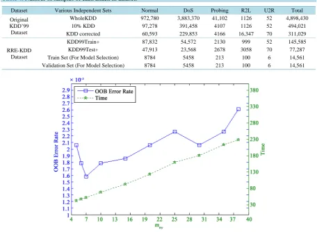
Table 4. Number of samples of each attack in dataset.

Dataset Various Independent Sets Normal DoS Probing R2L U2R Total

Original KDD’99 Dataset

WholeKDD 972,780 3,883,370 41,102 1126 52 4,898,430 10% KDD 97,278 391,458 4107 1126 52 494,021 KDD corrected 60,593 229,853 4166 16,347 70 311,029

RRE-KDD Dataset

KDD99Train+ 87,832 54,572 2130 999 52 145,585 KDD99Test+ 47,913 23,568 2678 3058 70 77,287 Train Set (For Model Selection) 8784 5458 213 100 6 14,561 Validation Set (For Model Selection) 8784 5458 213 100 6 14,561

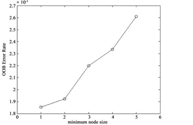
To determine the minimum node size, we use TrainSet for training and compare the OOB error rate with va-rying the number of node size with keeping ntree = 100 and mtry = 7, as shown in Figure 3. The plot shows that default value 1 (one) for classification gives the lowest OOB error rate.

6. Measure of Variable Importance and Variable Section

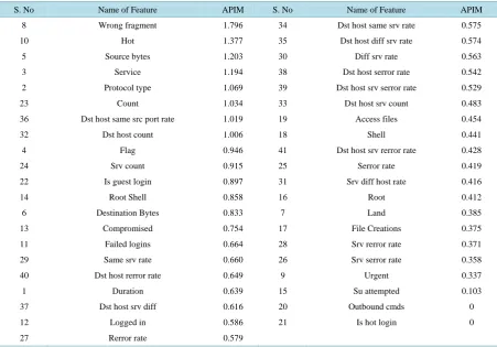
We run the Algorithm 1 to find out the APIM score of each feature and, also to analyze the feature relevancy in the training set. To run the Algorithm 1 (step one), we use the whole train dataset (KDD99Train+) with the val-ue of ntree = 100 and mtry = 7 those have been found in Section 5. Table 5 shows the details of the importance of each feature based their APIM score. The feature having higher APIM score is ranked high as shown in Table 5. After getting the sorted 41 features according to the APIM score, we run Algorithm 2 to select the best subset among 41 features. For every subset according to sorted order,, the whole train dataset (KDD99Train+) are used for RF and finally, we test the model by using the test dataset (KDD99Test+). As shown in Figure 4, where the

Figure 2. Comparison of training, Out-of-Bag, and independent test set error rates for random forest vs the number of trees.

Table 5. APIM scores are sorted for all the 41 features.

S. No Name of Feature APIM S. No Name of Feature APIM

8 Wrong fragment 1.796 34 Dst host same srv rate 0.575

10 Hot 1.377 35 Dst host diff srv rate 0.574

5 Source bytes 1.203 30 Diff srv rate 0.563

3 Service 1.194 38 Dst host serror rate 0.542

2 Protocol type 1.069 39 Dst host srv serror rate 0.529

23 Count 1.034 33 Dst host srv count 0.483

36 Dst host same src port rate 1.019 19 Access files 0.454

32 Dst host count 1.006 18 Shell 0.441

4 Flag 0.946 41 Dst host srv rerror rate 0.428

24 Srv count 0.915 25 Serror rate 0.419

22 Is guest login 0.897 31 Srv diff host rate 0.416

14 Root Shell 0.858 16 Root 0.412

6 Destination Bytes 0.833 7 Land 0.385

13 Compromised 0.754 17 File Creations 0.375

11 Failed logins 0.664 28 Srv rerror rate 0.371

29 Same srv rate 0.660 26 Srv serror rate 0.358

40 Dst host rerror rate 0.649 9 Urgent 0.337

1 Duration 0.639 15 Su attempted 0.103

37 Dst host srv diff 0.616 20 Outbound cmds 0

12 Logged in 0.586 21 Is hot login 0

27 Rerror rate 0.579

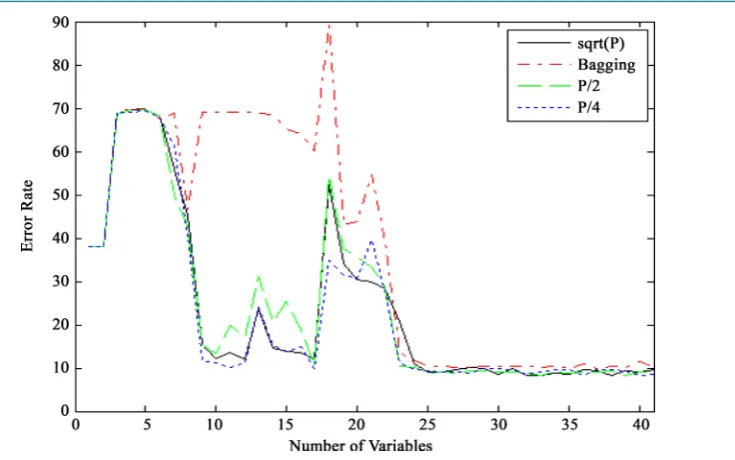
test error rates for each of the subset selected from the sorted 41 variables are calculated for various choices of mtry and a fixed choice of ntree = 100. The four different choices of mtry those we examined here are mtry = P, P/2, P/4, and P1/2, where the value of P is the number of features for each subset.

From Figure 4, it is clear that the test error rate remains roughly constant, if, at least, 25 descriptors are con-sidered, however, this figures also shows that consideration of descriptors more than 25 do not have significant effect on test error rate. Therefore, in our work, we select 25 variables which are listed in Table 6. Besides this, it is observed that the performance of various mtry, the default (sqrt(P)) one is usually the best, and bagging is the worst. Although, the default value of mtry is doing better, we again tune mtry for newly selected 25 variables by following the approach described in section 5 and we got the best performance at mtry = 8 and got the value of ntree = 100.

Finally, we take mtry = 8 and ntree = 100 for the selected 25 variables to train the whole train dataset (KDD99 Train+) as well as test the test dataset (KDD99Test+).

7. Results and Discussion

The final training/test phase is concerned with the development and evaluation on a test set of the final RF mod-el that is created based on the optimal hyper-parameters set found so far from the modmod-el smod-election phase [26]. After getting the parameters of RF with 41 features and selected 25 features as described in section 5 and 6 re-spectively, we build the model by using the whole train dataset (KDD99Train+) for the RF classifier and finally, we test the model by using the test dataset (KDD99Test+). The training and testing results are given in Table 7 according to the classification accuracy. From this Table 7, it is observed that the test accuracy for RF with 25 features is better than RF classifier with 41 variables. It is expected that reducing feature requires less time to train than to train with the whole feature, in our case, RF with 25 variables took less time than RF with 41 va-riables.

Figure 4. Test error rates versus the number of important variables, using different mtry.

Table 6. Selected 25 variables according to the APIM score.

Selected Feature According to Serial Number

1, 2, 3, 4, 5, 6, 8, 10, 11, 12, 13, 14, 22, 23, 24, 27, 29, 30, 32, 34, 35, 36, 37, 38, 40

Table 7. Training and testing accuracy.

Classifier Training Accuracy Testing Accuracy Train Time (min)

RF with 41 Features 100 91.41 10.62

RF with 25 Features 100 91.90 7.98

Table 8. Confusion matrix for random forest with 41 variables.

Actual

Dos Normal Probing R2L U2R %

Pr

ed

ictio

n

Dos 21795 55 185 0 0 98.91

Normal 1609 46585 231 2649 67 91.09

Probing 164 1272 2262 405 1 55.12

R2L 0 1 0 4 1 66.67

U2R 0 0 0 0 1 100

% 92.48 97.22 84.47 0.13 1.43

Table 9. Confusion matrix for random forest with 25 variables.

Actual

Dos Normal Probing R2L U2R %

Pr

ed

ictio

n

Dos 22196 56 181 0 0 98.94

Normal 1145 46424 213 2681 63 91.88

Probing 227 1344 2284 258 0 55.53

R2L 0 60 0 119 1 66.11

U2R 0 29 0 0 6 17.14

Table 10. False positive rate (%) of random forest for each of the attack types including normal.

Classifier Dos Normal Probing R2L U2R Average False Positive Rate

RF with 41 Variables 7.52 2.77 15.53 99.87 98.57 44.85

RF with 25 Variables 5.82 3.1 14.71 96.11 91.43 42.23

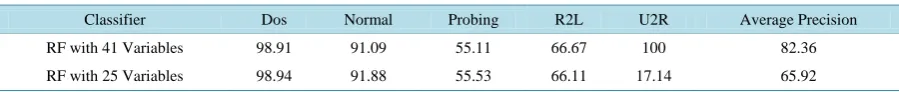
Table 11. Precision (%) of random forest for each of the attack types including normal.

Classifier Dos Normal Probing R2L U2R Average Precision

RF with 41 Variables 98.91 91.09 55.11 66.67 100 82.36

RF with 25 Variables 98.94 91.88 55.53 66.11 17.14 65.92

Going into more detail of the confusion matrix, it can be seen that RF with 25 variables performs better on all types of attack detection.

We also consider the false positive rate and precision for each of classifier and these are shown in Table 10 and Table 11, respectively. The RF with 41 variables gives high precision and on the other hand RF with 25 va-riables gives lower false positive rate.

8. Conclusion

In this paper, we presented a Random Forest model for Intrusion Detection Systems (IDS) with a focus on im-proving the intrusion detection performance by reducing the input features. From the context of real-world ap-plications, smaller numbers of features are always advantageous in terms of both data management and processing time. The obtained results indicate that the ability of the RF classification with reduced features (25 features) produces more accurate result than that of found from Random Forest classification with all features (41 features). Moreover, time required to process 25 features with RF is smaller than the processing time of RF with 41 features. The research in intrusion detection and feature selection using RF approach is still an ongoing area due to its good performance. The findings of this paper will be very useful for research on feature selection and classification. These findings can also be applied to use RF in more meaningful way in order to maximize the performance rate and minimize the false positive rate.

References

[1] Suebsing, A. and Hiransakolwong, N. (2011) Euclidean-Based Feature Selection for Network Intrusion Detection. In-ternational Conference on Machine Learning and Computing, 3, 222-229.

[2] Hasan, M.A.M., Nasser, M. and Pal, B. (2013) On the KDD’99 Dataset: Support Vector Machine Based Intrusion De-tection System (IDS) with Different Kernels. IJECCE, 4, 1164-1170.

[3] Adebayo, O.A., Shi, Z., Shi, Z. and Adewale, O.S. (2006) Network Anomalous Intrusion Detection Using Fuzzy-Bayes.

Intelligent Information Processing III, 525-530.

[4] Cannady, J. (1998) Artificial Neural Networks for Misuse Detection. National Information Systems Security Confe-rence, 368-381.

[5] Pal, B. & Hasan, M.A.M. (2012) Neural Network & Genetic Algorithm Based Approach to Network Intrusion Detec-tion & Comparative Analysis of Performance. 15th International Conference onComputer and Information Technolo-gy (ICCIT),Chittagong, 22-24 December 2012,150-154. http://dx.doi.org/10.1109/iccitechn.2012.6509809

[6] Hasan, M.A.M., Nasser, M., Pal, B. and Ahmad, S. (2014) Support Vector Machine and Random Forest Modeling for Intrusion Detection System (IDS). Journal of Intelligent Learning Systems and Applications, 6, 45.

http://dx.doi.org/10.4236/jilsa.2014.61005

[7] Wang, Q. and Megalooikonomou, V. (2005) A Clustering Algorithm for Intrusion Detection. Defense and Security, International Society for Optics and Photonics, 31-38.

[8] Chen, Y., Abraham, A. and Yang, J. (2005) Feature Selection and Intrusion Detection Using Hybrid Flexible Neural tree. Advances in Neural Networks—ISNN 2005, 3498, 439-444. http://dx.doi.org/10.1007/11427469_71

[9] Lee, W., Stolfo, S.J. and Mok, K.W. (1999) A Data Mining Framework for Building Intrusion Detection Models. Pro-ceedings of the 1999 IEEE Symposium onSecurity and Privacy, 120-132.

Sys-tems. Neural Information Processing, 3316, 1020-1025. http://dx.doi.org/10.1007/978-3-540-30499-9_158

[11] Chebrolu, S., Abraham, A. and Thomas, J.P. (2005) Feature Deduction and Ensemble Design of Intrusion Detection Systems. Computers & Security, 24, 295-307. http://dx.doi.org/10.1016/j.cose.2004.09.008

[12] Takkellapati, V.S. & Prasad, G.V.S.N.R.V. (2012) Network Intrusion Detection System Based on Feature Selection and Triangle Area Support Vector Machine. International Journal of Engineering Trends and Technology, 3, 466-470. [13] Chou, T.S., Yen, K.K. and Luo, J. (2008) Network Intrusion Detection Design Using Feature Selection of Soft

Compu-ting Paradigms. International Journal of Computational Intelligence, 4, 196-208.

[14] Lee, W., Stolfo, S.J. and Mok, K.W. (2000) Adaptive Intrusion Detection: A Data Mining Approach. Artificial Intelli-gence Review, 14, 533-567. http://dx.doi.org/10.1023/A:1006624031083

[15] Breiman, L. (2001) Random Forests. Machine learning, 45, 5-32. http://dx.doi.org/10.1023/A:1010933404324 [16] (2010) MIT Lincoln Laboratory, DARPA Intrusion Detection Evaluation. https://www.ll.mit.edu/ideval/data/

[17] (2010) KDD’99 Dataset. http://kdd.ics.uci.edu/databases

[18] Bahrololum, M., Salahi, E. and Khaleghi, M. (2009) Anomaly Intrusion Detection Design Using Hybrid of Unsuper-vised and SuperUnsuper-vised Neural Network. International Journal of Computer Networks & Communications (IJCNC), 1, 26-33.

[19] Singh, S. and Silakari, S. (2009) An Ensemble Approach for Feature Selection of Cyber Attack Dataset. arXiv preprint arXiv:0912.1014.

[20] Eid, H.F., Darwish, A., Hassanien, A.E. and Abraham, A. (2010) Principle Components Analysis and Support Vector Machine Based Intrusion Detection System. 10th International Conference onIntelligent Systems Design and Applica-tions (ISDA), 363-367.

[21] Tavallaee, M., Bagheri, E., Lu, W. and Ghorbani, A.A. (2009) A Detailed Analysis of the KDD CUP 99 Data Set.

Proceedings of the Second IEEE Symposium on Computational Intelligence for Security and Defence Applications

2009, Ottawa, 8-10 July 2009, 1-6. http://dx.doi.org/10.1109/CISDA.2009.5356528

[22] Liaw, A. and Wiener, M. (2002) Classification and Regression by Random Forest. R News, 2, 18-22.

[23] Svetnik, V., Liaw, A., Tong, C., Culberson, J.C., Sheridan, R.P. and Feuston, B.P. (2003) Random Forest: A Classifi-cation and Regression Tool for Compound ClassifiClassifi-cation and QSAR Modeling. Journal of Chemical Information and Computer Sciences, 43, 1947-1958. http://dx.doi.org/10.1021/ci034160g

[24] Sandri, M. and Zuccolotto, P. (2006) Variable Selection Using Random Forests. In: Zani, S., Cerioli, A., Riani, M. and Vichi, M., Ed., Data Analysis, Classification and the Forward Search, Springer, Berlin Heidelberg, 263-270.

http://dx.doi.org/10.1007/3-540-35978-8_30

[25] Qi, Y. (2012) Random Forest for Bioinformatics. In: Zhang, C. and Ma, Y.Q. Ed., Ensemble Machine Learning, Sprin- ger, US, 307-323.

http://dx.doi.org/10.1007/978-1-4419-9326-7_11