Solving the Carbon Dioxide Emission Estimation
Problem: An Artificial Neural Network Model
Abdel Karim Baareh
Computer Science Department, Ajloun College, Al-Balqa Applied University, Ajloun, Jordan. Email: [email protected]
Received May 9th, 2013; revised June 10th, 2013; accepted June 17th, 2013
Copyright © 2013 Abdel Karim Baareh. This is an open access article distributed under the Creative Commons Attribution License, which permits unrestricted use, distribution, and reproduction in any medium, provided the original work is properly cited.
ABSTRACT
Climate Pollution due to the Carbon Emission (CO2) from the different fossil fuels is considered as a great and impor-
tant international challenge to many researchers. In this paper we are providing a solution to forecast the poison CO2
gas emerged from energy consumption. Four inputs data were considered the global oil, natural gas, coal, and primary energy consumption to build our system. In this paper, we used the Artificial Neural Network (ANN) as successful and powerful tool in handling a time series modeling problem. The proposed ANN model was used to train and test the yearly CO2 Emission. The data were trained from year 1982 to 2000, and tested for the year 2003 to 2010. From the
results obtained we can see that ANN performance was Excellent and proved its efficiency as a useful tool in solving the climate pollution problems.
Keywords: Fossil Fuels; Carbon Emission; Forecasting; Artificial Neural Network; Back Propagation
1. Introduction
Forecasting the future events is a great, important and risky task that attracted many researchers in different fields. This type of problems contains many variables that should be studied, highlighted, and considered to build the suitable models. The world events and proc- esses should be clearly explained and obviously stated to be processed. Climate pollution due to the carbon emis- sion became an important and serious problem that af- fects the countries from the different aspects, health, cli- mate, agriculture, economics, and tourism. Adjusting the energy policies is a necessary process to void pollution problem, and keeping the atmosphere clear and clean [1]. All the future reading indicates the increase in CO2 and
greenhouse gas emission [2]. Many countries today have commitments between them to reduce the greenhouse gas emission, like the Kyoto protocol and the United Nations (UN) agreement to keep checking the CO2 emission per-
centage in the atmosphere in order to reduce it to the de- sired levels [3]. Many scientists consider the global warming due to CO2 emission is dangerous and threat the
world more than terrorism. Many countries such as the UK Government’s stated a clear objective in order to reduce the CO2emissions by 10% from the 1990 base by
2010 and in parallel to generate 10% of the UK’s elec-
tricity from renewable sources by 2010. Renewable elec- tricity has become equal with CO2 reduction [4]. Several
studies were developed to find out the relationship be- tween the different energy consumption and CO2 emis-
sion [5,6]. For all that there is a need to develop a non linear model that estimates the carbon dioxide emission. In this paper we used the artificial neural network as a powerful, capable tool in handling such type of modeling process. ANN was largely used in solving different pro- blems in numerous fields such as Rainfall-runoff, water quality, sedimentation and rainfall forecasting. ANN also proved its efficiency and strength in different number of applications [7,8] such as sales prediction [9], shift fail- ures [10], estimating prices [11] and stock returns [12]. In our case we explored the effect of four inputs vari- ables the global oil, natural gas (NG), coal, and primary energy (PE) consumption on the CO2 emission estima-
tion.
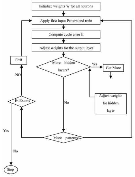
2. ANN Back Propagation Algorithm
reaching to the optimal weights numbers and values, reaching to the desired output from the given desired input. ANNs simulate the human biological nervous sys- tems, and the way it works is similar to the way the brain process information [13]. ANNs proved its strength and efficiency in solving numerous problems in different world fields such as business [14], forecasting [15], fea-ture extraction [16], classifications [17,18] etc. In this paper, we used the Back-propagation Neural Networks, which is the most popular and the well-known neural type [19,20]. Usually the ANNs architecture consists of three layers, the input layer, hidden layer and the output layer. The input layer receives the input from the outside world, where it has a number of neuron equal to the number of model input. The next layer is called the hid- den layer. This layer receives the input from the direct prior layers. The last layer is the output layer, used to produce the output as its name. Neurons in the same layer are not connected to each other but the neurons in each layer were fully connected to all neurons in the next layer. The neurons weights were adjusted using the acti- vation (i.e. sigmoid) function argument. This activation function is assumed to be nonlinear [21]. Let n1(p), n2(p),
···, nn(p) be the network inputs, and let md,1(p), md,2(p),···,
md,n (p) be the estimated output. The back propagation
neural network function can be also explained as [13]. 1) The output from the hidden layer is calculated using Equation (1).
sigmoid 1
θn
j i i ij
m p
n p w p j (1)Where wij are the weights between the input layer and
the hidden layer and between the hidden layer and the output layer, is a threshold value.
The sigmoid function is presented in Equation (2).
1 1 e jj n p
m p
(2)
The output from the output layer is calculated using Equation (3).
sigmoid 1
θn
j i i i j
m p
n p w p j (3)The Error Gradient from the output layer is calculated from Equation (4).
1
e
k p m pk m pk k p
(4)
where ek(p) is the error at the output layer
,
ek p md k p m pk
(5) 2) The ANNs weight can be computed as given in Equa- tion (6).
δ
jk j k
w p m p p
(6)
To readjust the weights of the ANNs we use Equation (7).
1
jk jk jk
w p w p w p
(7)The gradient error in the hidden layer is calculated from Equation (8).
1
δk j 1 j i δk jk
k
p m p m p p w p
(8)3) Calculating the weights again from Equation (9).
δ
ij i j
w p n p p
(9)4) A gain we readjust the weights by Equation (10).
1
ij ij ij
w p w p w p
(10)The back propagation algorithm can be simply ex-plained and shown from the flow chart in Figure 1.
3. Neural Network Model for Carbon
Emission Estimation Problem
[image:2.595.305.539.414.720.2]The neural network structure that used for the carbon es- timation is a multi-layer feed forward network. As ex- plained before the network consists of an input layer, one hidden layer, and an output layer. The input layer consists of four inputs data the global oil, natural gas, coal, and primary energy consumption. The hidden layer function is a nonlinear and consists of 5 neurons. The hidden units
are fully mapped and connected to both the input and output. The activation function of the hidden units pro- vides the network nonlinearity. The neurons optimal number of the hidden layer was selected by several trials. The network was trained using the Back Propagation (BP) algorithm. The number of neurons in hidden layer is se- lected to be 5. The output layer consists of one output neuron producing the corresponding carbon emission estimation. The output layer node has a linear activation function. The ANN developed models is shown in Fig- ure 2.
4. Proposed Model Structure and Evaluation
Criterion
In our case we used four inputs to estimate the CO2
emission. The inputs are: Oil (t-1), Oil (t-2), NG (t-1), NG (t-2), Coal (t-1), Coal (t-2), PE (t-1), PE (t-2) and the output is the CO2 (t), where the inputs are measured in
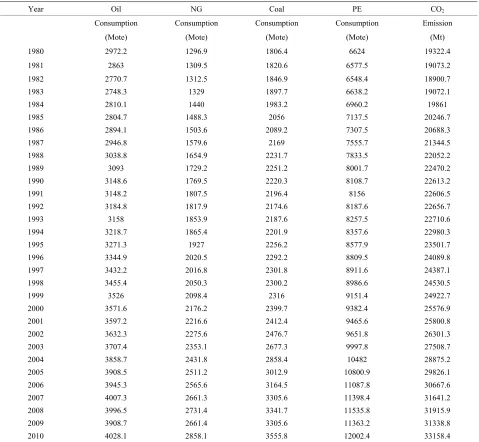
(Mote) and the output is measured in (Mt). The proposed network architecture was able to produce a very excellent estimation results in both training and testing cases with a very small number of differences. The neural network has 5 neurons in the hidden layers and one neuron in the output layer. The values of global oil, natural gas, coal, and primary energy consumption were obtained from [5,22]. The data in Table 1 were trained from the year 1982 to year 2000, and tested for the year 2003 to year 2010. In this paper we used different validation criterion to find out the percentage of error difference between the actual and estimated values as shown in Equations (11)- (13).
Manhattan distance
1
MD n i i
i
y y
(11)
Euclidian distance
2
1
ED n i i
i
y y
(12)
Mean magnitude of relative error
1 1 MMRE
i i N
i i
y y
N y
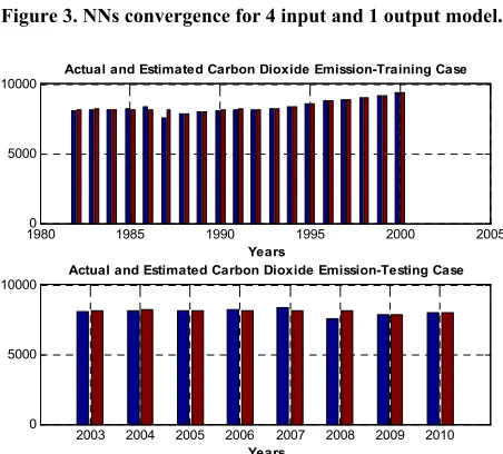
(13)where y and are the actual and estimated values based on the proposed model and N is the number of measurements used in the experiment, respectively. The neural network back propagation learning algorithm was able to perform the task properly by propagating the error each time reaching to the minimum error difference be- tween the actual and the estimated values. In Figure 3, we show The ANN convergence curve. Figure 4 shows the actual and estimated values in both training and test-
ing cases. The actual and estimated values were pre- sented in bar forms where blue bars are the actual values and red bars are the estimated one. The different valida- tion criteria performance evaluations are shown in Table 2.
y
5. Conclusion
In this study, we proposed an Artificial Neural Network
Oil(t-1) Oil(t-2) NG(t-1) NG(t-2) Coal(t-1) Coal(t-2) PE(t-1) PE(t-2) Co2(t-1)
[image:3.595.311.539.197.314.2]Co2(t)
[image:3.595.311.539.346.497.2]Figure 2. Developed neural network structure.
Figure 3. NNs convergence for 4 input and 1 output model.
19800 1985 1990 1995 2000 2005
5000 10000
Years
Actual and Estimated Carbon Dioxide Emission-Training Case
2003 2004 2005 2006 2007 2008 2009 2010 0
5000 10000
Years
[image:3.595.310.536.503.707.2]Actual and Estimated Carbon Dioxide Emission-Testing Case
Table 1. The data values of global oil, natural gas, coal, primary energy consumption and CO2emission [22].
Year Oil NG Coal PE CO2
Consumption Consumption Consumption Consumption Emission (Mote) (Mote) (Mote) (Mote) (Mt)
1980 2972.2 1296.9 1806.4 6624 19322.4 1981 2863 1309.5 1820.6 6577.5 19073.2 1982 2770.7 1312.5 1846.9 6548.4 18900.7
1983 2748.3 1329 1897.7 6638.2 19072.1
1984 2810.1 1440 1983.2 6960.2 19861
1985 2804.7 1488.3 2056 7137.5 20246.7
1986 2894.1 1503.6 2089.2 7307.5 20688.3
1987 2946.8 1579.6 2169 7555.7 21344.5
1988 3038.8 1654.9 2231.7 7833.5 22052.2 1989 3093 1729.2 2251.2 8001.7 22470.2 1990 3148.6 1769.5 2220.3 8108.7 22613.2 1991 3148.2 1807.5 2196.4 8156 22606.5 1992 3184.8 1817.9 2174.6 8187.6 22656.7 1993 3158 1853.9 2187.6 8257.5 22710.6 1994 3218.7 1865.4 2201.9 8357.6 22980.3
1995 3271.3 1927 2256.2 8577.9 23501.7
1996 3344.9 2020.5 2292.2 8809.5 24089.8 1997 3432.2 2016.8 2301.8 8911.6 24387.1 1998 3455.4 2050.3 2300.2 8986.6 24530.5
1999 3526 2098.4 2316 9151.4 24922.7
2000 3571.6 2176.2 2399.7 9382.4 25576.9 2001 3597.2 2216.6 2412.4 9465.6 25800.8 2002 3632.3 2275.6 2476.7 9651.8 26301.3 2003 3707.4 2353.1 2677.3 9997.8 27508.7 2004 3858.7 2431.8 2858.4 10482 28875.2 2005 3908.5 2511.2 3012.9 10800.9 29826.1 2006 3945.3 2565.6 3164.5 11087.8 30667.6 2007 4007.3 2661.3 3305.6 11398.4 31641.2 2008 3996.5 2731.4 3341.7 11535.8 31915.9 2009 3908.7 2661.4 3305.6 11363.2 31338.8 2010 4028.1 2858.1 3555.8 12002.4 33158.4
Table 2. MD, ED and MMER for ANN model training and testing data of the carbon estimation.
Model MD ED MMRE Training 61.1885 614.2148 0.0078
Testing 125.6023 606.6500 0.0160
model to estimate the values of the carbon dioxide emit- ted. The ANN was trained by the backpropagation learn- ing algorithm. The proposed ANN model results show that ANN was capable of producing high estimation ca- pabilities. This is clearly seen from the obtained results and the shown relationship between the actual and esti- mated responses. Again the ANNs proved its ability in solving the carbon estimating problem from a given set
of examples. We plan to explore the use of other soft computing techniques to solve this problem such as fuz- zy logic and genetic programming.
REFERENCES
[1] M. R. Lotfalipour, M. A. Falahi and M. Ashena, “Eco- nomic Growth, CO2 Emissions, and Fossil Fuels Con-
sumption in Iran,” Energy Policy, Vol. 2010, No. 35, 2010, pp. 5115-5120.
[2] H. Davoudpour and M. S. Ahadi, “The Potential for Greenhouse Gases Mitigation in Household Sector of Iran: Cases of Price Reform/Efficiency Improvement and Sce- nario for 2000-2010,” Energy Policy, Vol. 34, No. 1, 2006, pp. 40-49.
[image:4.595.56.287.584.628.2]dium-Term Forecasting of Anthropogenic Carbon Diox- ide and Methods Emission in Russia with Statistical Methods,” Vol. 34, No. 6, 2009, pp. 348-353.
[4] W. David, “Reduction in Carbon Dioxide Emissions: Estimating the Potential Contribution from Wind Power,” Renewable Energy Foundation, December 2004. [5] M. A. Behrang,. E. Assareh, M. R. Assari and A. Ghan-
barzadeh, “Using Bees Algorithm and Artificial Neural Network to Forecast World Carbon Dioxide Emission,”
Energy Sources, Part A: Recovery, Utilization, and Envi-
ronmental Effects, Vol. 33, No. 19, 2011, pp. 1747-1759.
[6] H. T. Pao and C. M. Tsai, “Modeling and Forecasting the CO2 Emissions, Energy Consumption, and Economic
Growth in Brazil,” Energy, Vol. 36, No. 5, 2011, pp. 2450-2458.
[7] N. Karunanithi, W. Grenney, D. Whitley and K. Bovee, “Neural Networks for River Flow Prediction,” Journal of
Computing in Civil Engg, Vol. 8, No. 2, 1993, pp. 371-
379.
[8] P. R. Bulando and J. Salas, “Forecasting of Short-Term Rainfall Using ARMA Models,” Journal of Hydrology, Vol. 144, No. 1-4, 1993, pp. 193-211.
[9] H. Hruschka, “Determining Market Response Functions by Neural Networks Modeling: A Comparison to Econo- metric Techniques,” European Journal of Operational
Research, Vol. 66, 1993, pp. 867-888.
[10] E. Y. Li, “Artificial Neural Networks and Their Business Applications,” Information and Managements, Vol. 27, No. 5, 1994, pp. 303-313.
[11] K. Chakraborty, “Forecasting the Behavior of Multivari- able Time Series Using Neural Networks,” Neural Net-
works, Vol. 5, 1992, pp. 962-970.
[12] G. Swales and Y. Yoon, “Applying Artificial Neural Net- works to Investment Analysis,” Financial Analyst Jour- nal, Vol. 48, No. 5, 1992, pp. 78-82.
[13] M. Negnevissky, “Artificial Intelligence: A Guide to Intelligent Systems,” 2nd Edition,Addison-Wesley, Bos- ton, 2005.
[14] E. Y. Li, “Artificial Neural Networks and Their Business
Applications,” Information and Managements, Vol. 27, No. 5, 1994, pp. 303-313.
[15] A. K. Baareh, A. Sheta and K. Al Khnaifes, “Forecasting River Flow in the USA: A Comparison between Auto- Regression and Neural Network Non-Parametric Mod- els,” Journal of Computer Science, Vol. 2, No. 10, 2006, pp. 775-780.
[16] M. S. Al-Batah, I. Mat, K. Z. Zamli and K. A. Azizli, “Modified Recursive Least Squares Algorithm to Train the Hybrid Multilayered Perceptron (HMLP) Network,”
Applied Soft Computing, Vol. 10, No. 1, 2010, pp. 236-
244.
[17] M. Seethe, I. V. Muralikrisha and B. L. Deekshatulu, “Artificial Neural Networks and Other Methods of Image Classifications,” Journal of Theoretical and Applied In-
formation Technology, Vol. 4, No. 11, 2005, pp. 1039-
1053.
[18] H. J. Lu, R. Setiono and H. Lui, “Effective Data Mining Using Neural Networks,” IEEE Transactions on Knowl-
edge and Data Engineering, Vol. 8, No. 6, 1996, pp. 957-
961.
[19] O. Kisi, “River Flow Modeling Using Artificial Net- works” Journal of Hydrologic Engineering, Vol. 9, No. 1, 2004, pp. 60-63.
[20] H. K. Cigizoglu and O. Kisi, “Flow Prediction by Three Back-Propagation Techniques Using K-Fold Partitioning of Neural Network Training Data,” Nordic Hydrology, Vol. 36, No. 1, 2005, pp. 49-64.
[21] A. K. Baareh, A. Sheta and K. Al Khnaifes, “Forecasting River Flow in the USA: A Comparison between Auto- Regression and Neural Network Non-Parametric Mod- els,” Proceedings of the 6th WSEAS International Con-
ference on Simulation, Modelling and Optimization, Lis-
bon, 22-24 September 2006, pp. 7-12.
[22] H. Kavoosi, M. H. Saidi, M. Kavoosi and M. Bohrng, “Forecast Global Carbon Dioxide Emission by Use of Genetic Algorithm (GA),” IJCSI International Journal of
Computer Science Issues, Vol. 9, No. 5, 2012, pp. 418-