The effect of energy consumption on countries’ economic efficiency: a conditional robust non parametric approach

(1)

Munich Personal RePEc Archive

The effect of energy consumption on

countries’ economic efficiency: a

conditional robust non parametric

approach

Halkos, George and Tzeremes, Nickolaos

University of Thessaly, Department of Economics

2011

Online at

https://mpra.ub.uni-muenchen.de/28692/

(2)

The effect of energy consumption on countries’

economic efficiency: a conditional robust non

parametric approach

by

George Emm. Halkos

1

and Nickolaos G. Tzeremes

Department of Economics, University of Thessaly, Korai 43, 38333, Volos, Greece

Abstract

This paper investigates the effect of energy consumption on countries’ economic efficiency. By using a sample of 18 EU countries for three census years (1980, 1990 and 2000) the paper employs conditional and unconditional robust nonparametric frontiers in order to establish such a relationship. By using probabilistic approaches it conditions the effect of energy consumption on the obtained countries’ economic efficiencies. With the use of nonparametric regressions the paper calculates the effect of energy consumption. The results reveal that lower levels of energy consumption increase countries’ economic efficiencies to a point where the effect of energy consumption on countries’ economic efficiency is neutral.

Keywords: Energy consumption; economic growth; robust efficiency estimators; conditional nonparametric techniques.

JEL Classification: Q43, O13, C6, C67

1

Associate Professor George Halkos Director of Postgraduate Studies Department of Economics, University of Thessaly,

Korai 43, 38333, Volos, Greece. http://www.halkos.gr

(3)

1. Introduction

The energy-growth relationship has been a popular topic for ‘old’ growth

theory and a on going debate for ‘new’ growth theory (van Zon and Yetkiner, 2003).

According to Moon and Son (1996) endogenous growth literature treats energy as

physical resource in an indirect ‘fashion’ which links higher economic growth with an

increased demand on energy. However several authors suggest that there is an

ongoing debate among the energy economists whether energy consumption can

stimulate economic growth and in which way (Gkali and El-Sakka, 2004;

Wolde-Rufael, 2005; Chontanawat et al., 2008). According to Stern (1993) and Beaudreau

(2005) energy is an essential factor of production. Moon and Sonn (1996) explain that

energy consumption increases productivity of other productive inputs in the

production process thus enhances economic growth. In contrast when energy

increases the investment in physical capital is decreased because the increased energy

use lowers the disposable income of the representative agent (p.194). Therefore, there

is a dynamic effect between these two forces which have an effect on energy

economic growth relationship. There have been many empirical studies explaining

this dynamic relationship in aggregated energy consumption (Soytas and Sari 2006,

2007) and in disaggregated levels (Shiu and Lam, 2004; Zhou and Chau, 2006) but

have presented mixed results. According to Yuan et al. (2008) the mixed results

which are reported in the literature are due to the fact that different countries are in

different developing stages. As such the developing process will have a different

impact on the relationship between energy consumption and economic growth. In an

extensive literature review Lee and Chang (2008) suggest that earlier studies have

examined the energy consumption – income/ output relationship mostly based in the

(4)

with Stern (1993, 2000) and Oh and Lee (2004) emphasizing that studies are based on

single countries or in small samples. As have been reported most of the studies, have

used panel data techniques and time series techniques such as cointegration and vector

error correction modeling in different countries for different time periods (Soytas and

Sari, 2006). In contrast, with those studies this paper adopts a different approach for

investigating the causal relationship between energy consumption and economic

growth. For the first time (to our knowledge) this paper uses robust non-parametric

frontiers (order-a) (Daouia and Simar, 2007) and its conditional form (Daraio and

Simar, 2005, 2007a,b) in order to establish the effect of energy consumption on

countries economic efficiency. By contributing to the existing literature this study

provides a framework of how the new advances in efficiency analysis can be applied

in order to for such a dynamic relationship to be investigated.

2. Literature review

Most of empirical studies examining the relationship between energy

consumption and economic growth in an aggregated and disaggregated level have

been inspired by the pioneered work by Kraft and Kraft (1978). By using data for a

time period of 1947 -1974 for the United States they found a unidirectional causality

from gross national product GNP to energy consumption. As such any energy policy

innervations wouldn’t affect GNP growth. However, Kraft and Kraft suggested that

this outcome was due to the selected time period. Similarly, Schurr (1982) examining

the period 1920 -1953 found that that in the United States the energy intensity of

production was falling while the country’s productivity was rising. However, for the

time period of 1953 -1973 energy intensity was stable while evidence indicated that

(5)

research remains to be done until will be able to establish the relationship between

energy utilization in productivity growth.

More recently, Lee and Chang (2008) examined the relationship between

energy consumption and real GDP within a multivariate framework which included

capital stock and labor as inputs for a sample of 16 Asian countries for the time period

of 1971-2002. By applying panel unit root, heterogeneous panel cointegration and

panel –based error correction models they found a long-run unidirectional causality

running from energy consumption to economic growth. In addition Mishra et al.

(2008) by testing for Granger causality and using panel cointegration techniques

examined the relationship between energy consumption and GDP for the Pasific

Island countries for the time period 1980-2005. Their evidence support that there is a

positive impact between energy consumption and GDP. In addition many studies have

used Granger causality tests in order to establish the link between energy and income

(Abosedra and Baghestani, 1991; Akarca and Long, 1980; Bentzen and Engsted,

1993; Hwang and Gum, 1992; Yu and Choi, 1985; Yu and Hwang, 1984). However,

the results reported are varying according to the country and the time period under

examination. Erol and Yu (1987) support this view by providing mixed results of a

sample of six countries. Similarly Stern (1993) found no evidence supporting that

gross energy use causes GDP. However, recent studies by adopting new time series

methodologies such as cointegration and vector error correction modelling couldn’t

establish a causal relationship between energy consumption and GDP growth. (Oh

and Lee, 2004; Soytas and Sari, 2006, 2007; Stern, 1993, 2000). Furthermore, van

Zon and Yetkiner (2003) reported that rising real energy prices tend to slow down

growth. Smulders and de Nooij (2003) developed a growth model in which growth is

(6)

found that energy conversation policies studied reduce per capita income levels. They

also found that in the long run energy policies which reduce energy tend to reduce

long run growth. According to Lee and Chang (2008) different sample data, different

techniques and different time periods have yield to inconsistent results of the energy –

economic growth relationship.

The problem of establishing the role of energy in the production process and

thus its causality relationship with GDP is a non ending academic debate over the last

three decades. Berndt and Wood (1975, 1979) using a time series data for US

economy have argued that energy and capital are compliments and energy and labour

are substitutes. In the same lines Hudson and Jorgenson (1974) and Solow (1987)

have also in favor of energy – capital complementarity. However Griffin and Gregory

(1976) and Joregenson and Wilcoxen (1990) have obtained results proving that

energy and capital are substitutes. In addition Smulders and de Nooij (2003) suggest

that labour and energy inputs are gross complements and are being combined with

specific complementary intermediate inputs which in turn are interpreted as capital in

the production function.

As such in contrast with the rest of the studies analysing the relationship

between energy consumption and economic growth, this paper for the first time uses

nonparametric techniques in order to establish the effect of energy consumption on

the economic efficiency of 18 EU countries for the period of three census years

(1980,1990 and 2000). In our paper we model and we measure countries’ economic

efficiency by adopting robust non-parametric frontiers (order-a) as has been

introduced by Daouia and Simar (2007). According to Daraio and Simar (2007a) the

use of robust frontiers are more robust to extreme values and outliers and thus we can

(7)

their determinist nature. In addition robust frontiers are not suffering from

dimensionality problems thus we can work with samples of small/ moderate sizes.

According to Daraio and Simar (2007a) order-a frontiers (used in this study) are more

robust to extremes than the order-m frontiers developed by Cazals et al. (2002). After

measuring countries’ economic efficiency levels we condition them to their energy

consumption levels for the examined period by using conditional robust frontiers

(Daraio and Simar, 2005, 2007b). The main advantage of robust ratios is that they can

show us the impact of energy consumption on countries’ economic efficiencies even

if we have in our sample some extreme observations (caused by countries’

heterogeneity). As such by treating energy consumption as an environmental factor

which influences countries’ process of economic activity we will be able to determine

robust conditional measures (conditioned to energy consumption) and thus to evaluate

if countries’ energy consumption levels for the examined periods had any effect on

their economic efficiencies.

3. Data

In the literature nonparametric techniques have been used to measure

countries’ environmental performance based on the production process (Färe et al.,

1989a,b; Chung et al., 1997; Zaim and Taskin, 2000; Taskin and Zaim, 2000; Zaim et

al., 2001; Zaim, 2004). However, non of the above studies have examined the

energy-GDP relationship using non parametric techniques. Following Halkos and Tzeremes

(2009a, b) we measure countries economic efficiency based in production of two

inputs and one output. We use data for three census years 1980, 1990 and 2000 for 18

European countries2. The inputs used are Total Fixed Investment (TFI) (excluding

stockbuilding) in volumes and Labour Force (LF) whereas the output used is the

2

(8)

Gross Domestic Product (GDP) (market prices) in volumes. The inputs/ output used

have been obtained from Economics Web Institute (EWI, 2009). The external variable

used is Primary Energy Consumption (PEC). Primary energy comprises commercially

traded fuels only. The energy consumption quantities have been obtained from BP

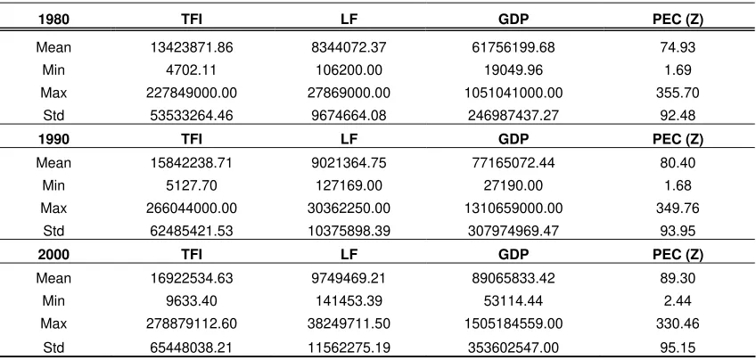
Statistical Review of World Energy (2007). Table 1 provides the descriptive statistics

of the inputs/ output used. As can be realised the energy consumption of the examined

countries have been examined over the years. Furthermore, the descriptive statistics

indicate that there are heterogeneities between the 18 countries. The heterogeneities

reported in GDP, labour and total fixed investment makes the methodology adopted

more appropriate since robust frontiers can accommodate samples with extreme

values.

Table 1 about here 4. Methodology

4.1Probabilistic approach to efficiency measurement

Daraio and Simar (2005) following extending the ideas of robust

measurements introduced by Cazals et al. (2002) introduced a probabilistic approach

of production process. Following the notation by Daraio and Simar (2007a) the

production set Ψ defined as a set of p inputs and q outputs in a Euclidean space R₊p+q

as:

( )

⎭ ⎬ ⎫ ⎩

⎨

⎧ _∈ _∈

=

Ψ x,y x R₊p,y R₊q,(x,y) is feasible (1),

where x is the input vector y the output vector. Then the production process can be

described by the joint probability measure of (X,Y) on R₊pxR₊q. Then the knowledge of

(9)

) , ( Pr ) ,

(x y ob X x Y y

H_XY = ≤ ≥ (2).

Then for the input oriented case the efficiency score θ(x,y) for (x,y)∈Ψcan be

defined as:

{

( ) 0

} {

inf ( , ) 0

}

inf ) ,

(x y =

θ

F_X_Y

θ

xy > =

θ

H_X_Y

θ

x y >

θ

(3).

A nonparametric estimator can be defined by replacing F_X_Y(xy)by its empirical

version:

∑

= = ∧ ≥ ℑ ≥ ≤ ℑ = _n i i n

i i i

n Y X y Y y Y x X y x F 1 1 , ) ( ) , ( )

( (4),

where ℑis the indicator function. Under the free disposal assumption the FDH

estimator of θ(x,y)developed by Deprins et al. (1984) coincides with the input

efficiency score for a given point (x,y) (Cazals et al., 2002):

⎭ ⎬ ⎫ ⎩ ⎨ ⎧ _> = ⎭ ⎬ ⎫ ⎩ ⎨

⎧ _∈_Ψ

= ∧ ∧ ∧ 0 ) ( inf ) , ( inf ) ,

(x y x y FDH FXY,n xy

FDH θ θ θ θ

θ (5).

4.2 The formulation of Order-a frontiers

Following Daouia and Simar (2007) an order- α nonparametric estimator can

be calculated as:

⎭ ⎬ ⎫ ⎩

⎨

⎧ _> ₋

= ∧ ∧ a y x F y

x XYn

n

a, ( , ) inf θ , (θ ) 1

θ (6).

According to Daraio and Simar (2007a) order-α quantile frontiers benchmark

the unit at (x,y) against the input level not exceed by (1-α) x 100% of the countries

among the population of units producing output levels of at least y. When, a→1 then

( )

x y FDH

( )

x y

n

a, , ,

∧ ∧

→θ

θ (5). The estimator a,n(x,y)

∧

θ can take values >,< and = to 1.

When )a,n(x,y

∧

(10)

inputs by a factor θ_α(x,y) to reach the same frontier. If θ_α(x,y)=1 then the countries is

said to be efficient at the level a x 100% since it is dominated by countries

producing more outputs than y with a probability 1-α. If θ_a(x,y)<1, then the country

(x,y) has to reduce its input to the level θ_a(x,y)x to reach the input efficient frontier

of level a x 100%.

4.3 Conditional Order-a frontiers

As has been described by Daraio and Simar (2005) different variables

(exogenous to the production process) Ζ∈ℜr can be used to explain the efficiency

variations of the production process. The idea is to condition the production process to

a given value of Z =z. The joint distribution (X,Y) conditional on Z =zdefines the

production process if Z = z. Then a nonparametric estimator θ_m(x,yz) is provided

by plugging the non parametric estimator:

∑

= = ∧ − ≥ ℑ − ≥ ≤ ℑ = _n

i i i

n

i i i i

n Z Y X h z z K y y h z z K y y x x z y x F 1 1 , , ) / ) (( ) ( ) / ) (( ) , ( ) ,

( (7),

where K(.) is the kernel and h is the bandwidth of appropriate size. We have used

kernel with compact support (Epanechnikov) as suggested by Daraio and Simar

(2005). Furthermore, for the calculation of bandwidth we used the two stage data

driven approach as proposed by Daraio and Simar (2006). As a first step we used the

likelihood cross validation criterion based on K-NN method (Silverman, 1986). As a

second step we take into account for the dimensionality of x and y, and the sparsity of

points in larger dimensional spaces we expand the local bandwidths hZi by a

factor1+n−1/(p+q), increasing with (p + q) but decreasing with n. In the second step

Similarly, following Daouia and Simar (2007) a conditional order-a nonparametric

(11)

⎪ ⎪ ⎪ ⎩ ⎪⎪ ⎪ ⎨ ⎧ − = < − ≤ < − ≤ = ₊ ₊ ∧ . 1 ,..., 1 1 1 0 ) ,

( ₁ ₁

1 ) 1 ( , y k k y k y n a M k l a l if X l a if X z y x

θ (8).

According to Daraio and Simar (2007a, 2007b) the global influence of Z on

the production process can be obtained by comparing the conditional order-a frontiers

to their unconditional equivalents. In a univariate case of Z a scatter-plot of the ratios

) , ( ) , ( , y x z y x Q a a z a ∧ ∧ = θ θ

against Z and its smoothed nonparametric regression line would

indicate the global effect of Z o the production process. If the smoothed

nonparametric regression is increasing it indicates that Z is unfavourable to efficiency

and when this regression is decreasing then is favourable to efficiency. Finally, we

use a nonparametric regression estimator introduced by Nadaraya (1964) and Watson

(1964):

∑

= = ∧ − − = n i i n i i h Z z K Q h Z z K z g 1 1 ) ( ) ( )

( (9).

4.4 Decomposition of conditional efficiency

We decompose the conditional efficiency obtained as suggested by Daraio and

Simar (2006). The conditional efficiency CEz(x,y)obtained for every country can be

decomposed in to three main indicators. The first indicator is the indicator of

unconditional efficiency UE(x,y) or countries’ internal efficiency. The second is the

(12)

value of the ratios Q_a_,_z given the value of z owned by the country. It is given by the

nonparametric fitted value of Q_a_,_z obtained by some appropriate nonparametric

regression of Q_a_,_z on Z:

(

)

(

)

(

)

(

)

∑

= = ∧ − − = = _n i i n

i azi i

z a h z z K h z z K Q z Z Q E 1 1 , , / / (10).

Where K(.)is the Kernel and h an appropriate bandwidth. Finally, the third

indicator is the individual index IIz(x,y) and can be defined as:

(

Q Z z

)

E

Q_a_z _a_z = ∧

,

, / (11).

The individual index measures country’s intensity in catching the

opportunities or threats by the external factor.

The formulation of the three index can be defined as:

) , ( * ) , ( * ) , ( ) ,

(x y UE x y EI x y II x y

CE = z z (12).

The decomposition of conditional efficiency give us the possibility for

analysing individual and localized effects of external factors (in our case energy

consumption) and interpret them together with their global influence on countries’

economic efficiency.

4. Empirical results

The analysis has been conducted in two stages for 1980, 1990 and 2000. As

such the conditional and unconditional measures have been obtained. The value of α

used in our analysis was 0.9. With values of α greater than 0.9 the efficiency scores

of order-a frontiers quickly converge to the estimates obtained by FDH frontier (see

equation 5). According to Daraio and Simar (2007a) when the order-a values are close

(13)

obtained from our analysis. For the year 1980 we realize the countries with higher

economic efficiency are Belgium, Greece, Italy, Spain and Portugal. The lowest

efficiency scores have been observed for Luxemburg, Iceland and Ireland. When we

took into account the effect of energy consumption for that year then countries’

economic efficiency scores have changed (for some cases). For instance Finland has

increased its economic efficiency performance from 0.64 to 0.74. Furthermore, Spain

has dramatically increased its economic performance from 1 to 2.853. Similarly,

France has also been increased its economic efficiency from 0.61 to 1. In contrast

with Greece which under the influence of energy consumption its economic efficiency

has been decreased from 1 to 0.85. The same stands for Netherlands which had a

decrease from 0.63 to 0.31.

Table 2 about here

Continuing in the same way our analysis for 1990 we realise that in some

cases the effect of energy consumption caused an increase of countries’ economic

efficiencies and in some cases caused even a decrease of their economic efficiencies.

However as have been also reported for year 1980 when examine countries

efficiencies of 1990, we realise that in some cases energy consumption hadn’t any

effect on countries economic efficiency performances. For instance Germany in both

years is reported to have the same economic efficiency score regardless the effect of

energy consumption. The same goes for Iceland, Belgium and Ireland. Lee and Chang

(2008) suggest that the findings of no causality in either direction is called ‘neutrality

hypotheses’ and signifies no effect of energy consumption on countries growth. In

addition for the year of 1990 we can observe for the case of Austria a high increased

of its economic efficiency (from 0.27 to 0.77). The same goes for Denmark which had

3

(14)

an increase of its efficiency from 0.54 to 1.However, the highest decreases of

countries economic efficiencies have been reported for Sweden (from 0.85 to 0.23)

and the United Kingdom (from 0.72 to 0.39). Finally, when looking the results

obtained for the year 2000 we can realise that in some cases countries’ efficiency

scores haven’t been affected by the countries’ energy consumption levels (Belgium,

Germany, Iceland, Ireland, Italy and Spain). Again for some cases we observe an

increase of their economic efficiency scores (Austria, Denmark, Finland, France, and

Portugal) and for some we observe a decrease (Netherlands, Luxembourg, Norway,

Sweden, Switzerland and the United Kingdom). As can be realised the effect of

energy consumption on countries’ economic efficiency is change over the years under

examination and among the countries themselves. Even though our sample contains

phenomenically same countries (EU members) we observe that the effect of energy

consumption in some cases changes rapidly even if we examine the same country (see

for instance the case of Austria, Sweden, Finland and the United Kingdom). In fact

this phenomenon explains the dynamics between energy demand and economic

growth which have a counteracting relationship (Monn and Sonn, 1996).

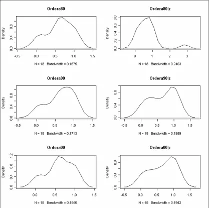
Figure 1 about here

In an aggregative way figure illustrates the density of the conditional and

unconditional efficiency scores of the 18 EU countries. As can be realised for the year

1980 countries’ energy consumption seem to have a positive effect on their economic

efficiencies concentrating their economic efficiency levels around unity. However,

when looking the year of 1990, we realise that the effect of energy consumption had

rather a negative/ neutral effect forcing countries’ economic efficiency scores away

from unity (left asymmetry, i.e. the median is greater than the mean). The same can be

(15)

scores is observed indicating that the effect of energy consumption is neutral and in

some cases negative. According to Monn and Son (1996) the increased energy use

lowers the disposal income of the representative agents, thus a decrease on investment

of physical capital is observed which in turn has a negative effect on countries’

economic efficiencies.

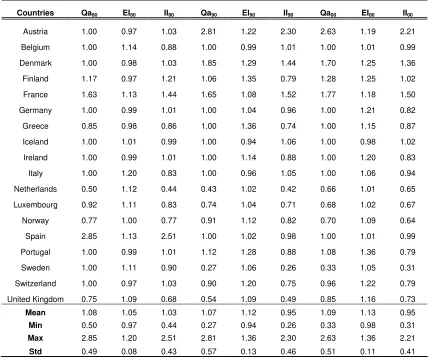
Table 3 about here

In order to analyse further the effect of energy consumption on countries’

economic efficiencies we decompose the conditional efficiency as have been

proposed by Daraio and Simar (2006). Table 3 provides the results of the conditional

efficiency decomposition in its components (see equation 12). The index Q_a is the

ratio of

) , (

y x

z y x

a a

∧ ∧

θ θ

and can take values >,<,=1. As such when Q_a is equal 1 indicates

that energy consumption has a neutral effect on country’s economic efficiency.

However, when the values are greater than 1 then the effect is positive and when are

lower than 1 the effects are negative. As can be observed for 1980 for the majority of

countries (Austria, Belgium, Denmark, Germany, Iceland, Ireland, Italy, Portugal,

Sweden and Spain) the energy consumption had a neutral effect on their economic

efficiency. In addition the externality index (EI) when takes values above 1 means

that the country works at a energy level with an expected Q_a >1. The opposite occurs

when EI takes values below1. As can be realised for the year 1980 the countries with

EI greater than unity are reported to be Belgium, France, Iceland, Italy, Netherlands,

Luxembourg, Spain, Sweden and the United Kingdom. However, in some cases the

effect of the energy consumption is not (as expected) positive. For instance Belgium

(16)

externality index is 1.12 but the value of Q_a is 0.5 indicating a negative effect of

energy consumption on country’s economic efficiency. This is maybe to

differentiations of energy prices among the observed countries or to different

consumption patterns and various sources of energy (Soytas and Sari, 2007). Finally,

the individual index (II80) analyses how the country performed in respect to the

expected value of its performance. For instance if individual index is greater than 1

then the effect of energy consumption on the efficiency score of the country under

consideration is higher with respect to its expected value. In contrast, if II <1 we are

considering a country for which the environmental externality (energy consumption)

is lower then what expected for its level of energy consumption. As such countries

with the expected higher influence (relative to their energy consumption) are reported

to be Austria, Denmark, Finland, France, Germany, Ireland, Spain, Portugal and

Switzerland. However, this expected influence is not reflected on their economic

efficiency scores. If continue our analysis in the same fashion for year 1990 we realise

that five countries have been positively influenced by their energy consumption, six

of them have been negatively influenced and seven of them had a neutral effect of

energy consumption on their economic efficiency. In addition when looking the year

2000 we realise that five countries have increased their economic efficiency as a

result of their energy consumption, whereas six of them have reduce their economic

efficiency scores. Finally, energy consumption appeared to have a neutral effect on

seven countries’ economic efficiencies. Again the disparities and differentiations of

energy prices, energy consumption patterns, macroeconomic policies and economic

process appeared to be a major obstacle for identifying a global effect of causality

between energy consumption and economic efficiency.

(17)

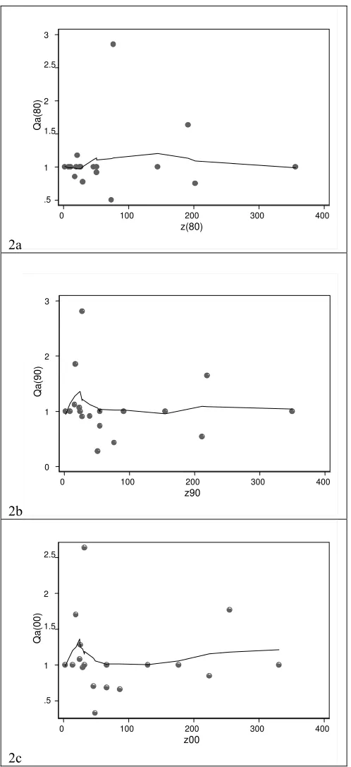
As described previously figure 2 illustrates the effect of energy consumption

on countries’ economic efficiency for the years 1980, 1990 and 2000 (subfigures

2a,b,c additionally). For instance subfigure 2a examines the influence of energy

consumption on countries’ economic performance for the period of 1980. It represents

a scatter plot of the ratios n

(

x,yz

)

/ n

( )

x,y

∧ ∧

θ

θ against countries’ energy consumption

levels and its smoothed nonparametric regression line in order to define this influence.

As the regression line is almost flat it specifies that energy consumption has a rather

neutral effect to the countries’ economic efficiencies. Accordingly for the year 1990

we realise at lower levels of energy consumption the effect is negative to the

countries’ economic efficiency levels bust when the energy consumption increases

again we realise that the effect is neutral. Finally, for the year 2000 we realise that in

lower levels of energy consumption the effect is negative but as the energy

consumption increases countries’ economic efficiencies are also increasing to a point

where the effect of energy consumption on countries’ economic efficiency is neutral.

As such our findings fully support previous studies by Lee and Chang (2008) and

Moon and Son (1996) which mention the difficulties and the dynamic nature of the

energy consumption-economic growth relationship.

5. Conclusions

As has been highlighted by several scholars (van Zon and Yetkiner, 2003;

Stern, 1993, 2000; Beaudreau, 2005; Smulders and de Nooij, 2003) the

energy-economic growth relationship is an ongoing debate among the energy economists. As

such any measures and techniques adopted must be critically evaluated and applied

before establishing the causality of such a dynamic relationship. To our knowledge

for the first time conditional and unconditional measures have been used in order to

(18)

well known studies employing advanced panel and time series techniques in

aggregated and disaggregated level (Soytas and Sari 2006, 2007; Shiu and Lam, 2004;

Zhou and Chau, 2006; Lee and Chang, 2008; Yuan et al., 2008; Stern, 1993 2000; Oh

and Lee, 2004, among others) this study uses order–a frontiers as introduced by

Daouia and Simar (2007). The results reveal that lower levels of energy consumption

have a negative effect on countries economic efficiency. This finding comes along

with the view by Smulders and Nooij (2003) suggesting that cuts in energy can have a

seriously affect on GDP and economic growth. Furthermore, the results reveal that

when the energy consumption values increase significantly can have a negative effect

on countries’ economic efficiencies. However, from a point onwards the effect of

energy consumption on countries’ economic efficiency is neutral. Lee and Chang

(2008) suggest that this finding is in the favour of the ‘neutrality hypothesis’ whereas

the negative effect on countries’ economic efficiencies may be as a result of a

decrease of disposable income of the representative agent due to increase in energy

prices of the countries under examination (Moon and Sonn, 1996).

As a limitation of the research provided may be the fact that we are examining

only three census years and having a sample of only 18 EU countries. In fact this must

be a direction for a future research; however, our intension was to highlight the

dynamics of the energy-economic growth relationship using the new advances in

nonparametric techniques. In contrast with the studies mentioned previously this

technique (especially with the decomposition of conditional efficiency) can provide us

with useful information of the insides and the structure of the energy consumption –

economic growth relationship in such a way that we will be able to overcome the

problems of countries’ dissimilarities.

(19)

6. References

Abosedra S, Baghestani H. Newevidence on the causal relationship between United

States energy consumption and gross national product. Journal of Energy and

Development 1991;14;285–292.

Akarca AT, Long TV. On the relationship between energy and GNP: A

reexamination. Journal of Energy and Development 1980; 5; 326–331.

Beaudreau BC. Engineering and economic growth. Structural Change and Economic

Dynamics 2005; 16; 211–220.

Bentzen J, Engsted T. Short- and long-run elasticities in energy demand. Energy

Economics 1993; 15; 9–16.

Berndt ER, Wood DO. Technology, prices and the derived demand for energy.

American Economic Review 1975; 56; 259–268.

Berndt ER, Wood DO. Engineering and econometric interpretations of energy capital

complementarity. American Economic Review 1979; 69; 342–354.

BP Statistical Review of World Energy June; 2007. Data can be obtained from

http://www.bp.com/statisticalreview (accessed September 13, 2009).

Cazals C, Florens JP and Simar L. Nonparametric frontier estimation: a robust

approach. Journal of Econometrics 2002; 106; 1-25.

Chontanawat J, Hunt LC and Pierse R. Does energy consumption cause economic

growth?: Evidence from a systematic study of over 100 countries. Journal of Policy

Modeling 2008; 30; 209–220.

Chung YH, Färe R and Grosskopf S. Productivity and undesirable outputs: a

directional distance function. Journal of Environmental Management 1997; 51; 229–

(20)

Daouia A, Simar L. Nonparametric Efficiency Analysis: A Multivariate Conditional

Quantile Approach. Journal of Econometrics 2007; 145; 375-400.

Daraio C, Simar L. A robust nonparametric approach to evaluate and explain the

performance of mutual funds. European Journal of Operational Research 2006; 175;

516–542

Daraio C, Simar L. Introducing Environmental Variables in Nonparametric Frontier

Models: a Probabilistic Approach. Journal of Productivity Analysis 2005; 24; 93-121.

Daraio C, Simar L. Advanced robust and nonparametric methods in efficiency

analysis. Springer Science: New York; 2007a.

Daraio C, Simar L. Conditional nonparametric frontier models for convex and

nonconvex technologies: a unifying approach. Journal of Productivity Analysis

2007b; 28; 13-32.

Deprins D, Simar L and Tulkens H 1984. Measuring labor-efficiency in post offices.

In Marchand M, Pestieau P and Tulkens H (Eds), The Performance of public

enterprises - Concepts and Measurement. North-Holland: Amsterdam, 1984. p. 243-

267.

Erol U, Yu ESH. On the causal relationship between energy and income for

industrialized countries. Journal of Energy and Development 1987; 13; 113–122.

EWI. Economics Web Institute; 2009. Data can be obtained from

http://www.economicswebinstitute.org (accessed September 13, 2009).

Färe R, Grosskopf S, Lovell CAK and Pasurka C. Multilateral productivity

comparisons when some outputs are undesirable. The Review of Economics and

(21)

Färe R, Grosskopf S and Pasurka C. The effect of environmental regulations on the

efficiency of electric utilities: 1969 versus 1975. Applied Economics 1989b; 21; 225–

235.

Ghali KH, El-Sakka MIT. Energy use and output growth in Canada: A multivariate

cointegration analysis. Energy Economics 2004; 26; 225–238.

Griffin JM, Gregory PR. An intercountry translog model of energy substitution

responses. American Economic Review 1976; 66; 845-847.

Halkos G, Tzeremes N. Measuring regional economic efficiency: the case of Greek

prefectures, The Annals of Regional Science 2009a; doi: 10.1007/s00168-009-0287-6.

Halkos G, Tzeremes N. Exploring the existence of Kuznets curve in countries'

environmental efficiency using DEA window analysis. Ecological Economics 2009b;

68; 2168-2176.

Hudson EA, Jorgenson DW. U.S. energy policy and economic growth, 1975-2000.

Bell Journal of Economics 1974; 5; 461-514.

Hwang DBK, Gum B. The causal relationship between energy and GNP: The case of

Taiwan. The Journal of Energy and Development 1992; 16; 219–226.

Jorgenson DW. The role of energy in productivity growth. American Economic

Review 1984; 74; 26-30.

Jorgenson DW, Wilcoxen PJ. Environmental regulation and US economic growth.

Rand Journal of Economics 1990; 21; 314–340.

Kraft J, Kraft A. On the relationship between energy and GNP. Journal of Energy

Development 1978; 3; 401-403.

Lee CC, Chang CP. Energy consumption and economic growth in Asian economies:

A more comprehensive analysis using panel data. Resource and Energy Economics

(22)

Mishra V, Smyth R and Sharma S. The energy-GDP nexus: Evidence from a panel of

Pacific Island countries, Resource and Energy Economics 2008;

doi:10.1016/j.reseneeco.2009.04.002

Moon YS, Sonn YH. Productive energy consumption and economic growth: An

endogenous growth model and its empirical applications. Resource and Energy

Economics 1996; 18; 189-200.

Nadaraya EA. On estimating regression. Theory of Probability Applications 1964; 9;

141-142.

Oh W, Lee K. Energy consumption and economic growth in Korea: testing the

causality relation. Journal of Policy Modeling 2004; 26; 973–981.

Schurr S. Energy efficiency and productive efficiency: Some thoughts based on

American experience. Energy Journal 1982; 3; 3-14.

Shiu A, Lee LP. Electricity consumption and economic growth in China. Energy

Policy 2004; 32; 47–54.

Silverman BW. Density estimation for statistics and data analysis. Chapman and Hall:

London; 1986.

Smulders S, de Nooij M. The impact of energy conservation on technology and

economic growth. Resource and Energy Economics 2003; 25; 59–79.

Solow JL. The capital energy complementarity debate revisited. American Economic

Review 1987; 77; 605–614.

Soytas U, Sari R. Can China contribute more to the fight against global warming?

Journal of Policy Modeling 2006; 28; 837–846.

Soytas U, Sari R. The relationship between energy and production: evidence from

(23)

Stern DI. Energy and economic growth in the U.S.A. Energy Economics 1993; 15;

137–150.

Stern DI. Multivariate cointegration analysis of the role of energy in the U.S.

macroeconomy. Energy Economics 2000; 22; 267–283.

Taskin, F., Zaim, O., 2000. Searching for a Kuznets curve in environmental efficiency

using kernel estimations. Economics Letters 68, 217–223.

van Zon A, Yetkiner IH. An endogenous growth model with embodied energy-saving

technical change. Resource and Energy Economics 2003; 25; 81-103.

Watson GS. Smooth regression analysis. Sankhya Series A 1964; 26; 359-372.

Wolde-Rufael Y. Energy demand and economic growth: The African experience.

Journal of Policy Modeling 2005; 27; 891–903.

Yu ESH, Hwang BK. The relationship between energy and GNP: Further results.

Energy Economics 1984; 6; 186–190.

Yu ESH, Choi JY. The causal relationship between energy and GNP: An international

comparison. Journal of Energy and Development 1985; 10; 249–272.

Yuan JH, Kang JG, Zhao CH, Hu ZG. Energy consumption and economic growth:

Evidence from China at both aggregated and disaggregated levels. Energy Economics

2008; 30; 3077–3094.

Zaim O. Measuring environmental performance of state manufacturing through

changes in pollution intensities: a DEA framework. Ecological Economics 2004; 48;

37–47.

Zaim O, Färe R, Grosskopf S. An economic approach to achievement and

improvement indexes. Social Indicators Research 2001; 56; 91–118.

Zaim O, Taskin F. A Kuznets curve in environmental efficiency: an application on

(24)

Zhou G, Chau KW. Short and long-run effects between oil consumption and

(25)

[image:25.595.87.511.96.298.2]

Table 1:Descriptive statistics of the variables used

1980 TFI LF GDP PEC (Z)

Mean 13423871.86 8344072.37 61756199.68 74.93

Min 4702.11 106200.00 19049.96 1.69

Max 227849000.00 27869000.00 1051041000.00 355.70

Std 53533264.46 9674664.08 246987437.27 92.48

1990 TFI LF GDP PEC (Z)

Mean 15842238.71 9021364.75 77165072.44 80.40

Min 5127.70 127169.00 27190.00 1.68

Max 266044000.00 30362250.00 1310659000.00 349.76

Std 62485421.53 10375898.39 307974969.47 93.95

2000 TFI LF GDP PEC (Z)

Mean 16922534.63 9749469.21 89065833.42 89.30

Min 9633.40 141453.39 53114.44 2.44

Max 278879112.60 38249711.50 1505184559.00 330.46

Std 65448038.21 11562275.19 353602547.00 95.15

(26)

[image:26.595.84.517.94.397.2]

Table 2: Conditional and unconditional efficiency scores

Countries ( , ) 80

y x

a

θ θ_a80(x,yz ) 90( , )

y x

a

θ θ_a90(x,yz ) 00( , )

y x

a

θ θ_a00(x,yz )

Austria 0.77 0.77 0.27 0.77 0.33 0.86

Belgium 1.00 1.00 1.00 1.00 1.00 1.00

Denmark 0.62 0.62 0.54 1.00 0.67 1.14

Finland 0.64 0.74 0.90 0.95 0.56 0.72

France 0.61 1.00 0.61 1.00 0.56 1.00

Germany 0.70 0.70 0.66 0.66 0.84 0.84

Greece 1.00 0.85 1.00 1.00 1.00 1.00

Iceland 0.04 0.04 0.05 0.05 0.06 0.06

Ireland 0.07 0.07 0.06 0.06 0.07 0.07

Italy 1.00 1.00 1.00 1.00 1.00 1.00

Netherlands 0.63 0.31 0.69 0.30 0.71 0.47

Luxembourg 0.06 0.06 0.06 0.05 0.07 0.05

Norway 0.58 0.45 0.47 0.43 0.54 0.38

Spain 1.00 2.85 1.00 1.00 1.00 1.00

Portugal 1.00 1.00 1.00 1.12 1.00 1.08

Sweden 0.21 0.21 0.85 0.23 0.57 0.19

Switzerland 0.57 0.57 0.64 0.58 0.59 0.57

United Kingdom 0.47 0.35 0.72 0.39 0.59 0.50

Mean 0.61 0.70 0.64 0.64 0.62 0.66

Min 0.04 0.04 0.05 0.05 0.06 0.05

Max 1.00 2.85 1.00 1.12 1.00 1.14

(27)

[image:27.595.83.514.97.457.2]

Table 3: Decomposition of the conditional efficiencies scores

Countries Qa80 EI80 II80 Qa90 EI90 II90 Qa00 EI00 II00

Austria 1.00 0.97 1.03 2.81 1.22 2.30 2.63 1.19 2.21

Belgium 1.00 1.14 0.88 1.00 0.99 1.01 1.00 1.01 0.99 Denmark 1.00 0.98 1.03 1.85 1.29 1.44 1.70 1.25 1.36

Finland 1.17 0.97 1.21 1.06 1.35 0.79 1.28 1.25 1.02

France 1.63 1.13 1.44 1.65 1.08 1.52 1.77 1.18 1.50

Germany 1.00 0.99 1.01 1.00 1.04 0.96 1.00 1.21 0.82

Greece 0.85 0.98 0.86 1.00 1.36 0.74 1.00 1.15 0.87

Iceland 1.00 1.01 0.99 1.00 0.94 1.06 1.00 0.98 1.02

Ireland 1.00 0.99 1.01 1.00 1.14 0.88 1.00 1.20 0.83

Italy 1.00 1.20 0.83 1.00 0.96 1.05 1.00 1.06 0.94

Netherlands 0.50 1.12 0.44 0.43 1.02 0.42 0.66 1.01 0.65 Luxembourg 0.92 1.11 0.83 0.74 1.04 0.71 0.68 1.02 0.67

Norway 0.77 1.00 0.77 0.91 1.12 0.82 0.70 1.09 0.64

Spain 2.85 1.13 2.51 1.00 1.02 0.98 1.00 1.01 0.99

Portugal 1.00 0.99 1.01 1.12 1.28 0.88 1.08 1.36 0.79 Sweden 1.00 1.11 0.90 0.27 1.06 0.26 0.33 1.05 0.31 Switzerland 1.00 0.97 1.03 0.90 1.20 0.75 0.96 1.22 0.79

United Kingdom 0.75 1.09 0.68 0.54 1.09 0.49 0.85 1.16 0.73

Mean 1.08 1.05 1.03 1.07 1.12 0.95 1.09 1.13 0.95

Min 0.50 0.97 0.44 0.27 0.94 0.26 0.33 0.98 0.31

Max 2.85 1.20 2.51 2.81 1.36 2.30 2.63 1.36 2.21

(28)

[image:28.595.90.509.72.486.2]

(29)

[image:29.595.84.333.91.634.2]

Figure 2: The Global effect of energy consumption on countries’ economic efficiencies

2a

2b

2c