Estimating Illumination Chromaticity Based on Structured Support Vector Machine

2016 International Conference on Computer, Mechatronics and Electronic Engineering (CMEE 2016) ISBN: 978-1-60595-406-6

Estimating Illumination Chromaticity Based

on Structured Support Vector Machine

Zheng TANG, Hong-zhe LIU*, Jia-zheng YUAN, Chao LI

and Yong-rong ZHENG

Beijing Key Laboratory of Information Service Engineering, Beijing Union University, Beijing 100101, China

*Corresponding author

Keywords: Color constancy, Multi-illuminant, White balance.

Abstract. Illumination estimation is crucial to the color constancy problem. Most existing color constancy algorithms assume uniform illumination. However, in real-world scenes, this is not often the case. Thus, we propose a novel framework for estimation the colors of multiple illuminants and their spatial distribution in the scene. We formulate this problem as an illuminant color estimate is obtained independently from distinct image main-regions. We think there is only one kind of light in each main-regions. From these main-regions a robust local illumination color is computed by consensus. So we can solve the problem of multiple illumination estimation using single illuminant color constancy method. The performance if our method is evaluated on multiple data sets. Experimental results show that we can reliably process mixed illuminant scenes.

Introduction

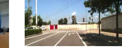
At present, most of the color constancy algorithm assumes that the scene illumination is evenly distributed in the whole scene; there is only one light value. In real life, however, there are often multiple illuminations in the scene, as shown in Figure 1. In indoor scenes, as shown in Figure 1(a), some areas are mainly indoor tungsten light source, and some areas are both indoor tungsten light and outdoor light source. As shown in Figure 1(b), an outdoor scene, where parts of the image are in direct sunlight, while others are in shadow which is illuminated by blue skylight. Color is one of the most basic features of machine vision, in the field of image processing and computer vision have been widely used, such as image segmentation, object recognition, image matching, video retrieval and others. The key to cancel out the effect of incident light is to estimate the color of the overall scene illumination. Unfortunately, color constancy is an ill-posed problem, so light color cannot be gained without any assumptions [1]. Because of the multi-illumination scene, the change of the illumination value will change with the change of its spatial position. In this case, if the assumption of scene illumination is uniform, and the use of single color under illumination condition estimation those. And based on the illumination value to correct the image color, will produce a lot of deviation, is not accurate to restore the surface color of the object. Compared with the single illuminant Chromaticity estimation, multiple color illumination estimation is more challenging. Extending existing color constancy methods to successfully compute multi-illuminant estimates is a challenging problem [14].

(a) indoor scene (b) outdoor scene

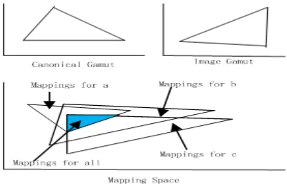
Consider two of the most popular branches of existing color constancy approaches: statistic-based methods and machine learning-based methods [14]. The success of statistics-based techniques [1], [2], [3], [4] depends on the size of the statistical sample. Applying these methods to small image regions introduces inaccuracies [5] and is unlikely to yield stable results. This kind of method originates from the Retinex theory [7], the color of objects is reflected by the object of long wave, medium wave, short wave to decide, rather than by the intensity of light. Based on the Retinex theory and algorithm, the researchers proposed the hypothesis of Grey World and Patch White hypothesis [6]. Patch White algorithm is based on the assumption of Patch White [7]. The maximum response in a scene is caused by a perfect reflectance. Because the white surface can completely reflect the color of the scene, so the maximum value of the RGB three color channels will be used as the image of the light color value [7]. Finlayson et al.[8] based on Grey World algorithm, P (Minkowski-norm) is introduced into the Grey-World algorithm, using P distance instead of simple averaging methods RGB color channels, and presents a general algorithm framework of Shades-of-Grey (SoG) algorithm, through changing the p value (0<P<∞), which contains White Patch and Grey World algorithm. Gamut mapping algorithm Forsyth proposed by [9], the assumption that any one image type light source color is limited, color channel RGB value after normalization in the color space is formed on a closed convex hull (convex hull) also known as color (Gamut), schematic diagram as shown in Figure 2 color gamut mapping:

Figure 2. Color gamut mapping space.

D.H. Brainard [4] proposed a color constancy algorithm based on Bayesian inference, after Rosenberg and Gehler made a series of improvements. Finlayson proposed a color constancy algorithm based on correlation (Color by Correlation) [9], the algorithm is more practical.

Based on machine learning for estimation the colors of multiple illuminants. Study the original method of color constancy machine is based on the neural network model [9], compared with the previous color constancy algorithm, neural network algorithm has superior performance [12], parallel processing speed is higher than the traditional algorithm with adaptive function [10]. According to the data provided by the sample to learn and find out the intrinsic link between the output data and the implicit law gradually come out. Methods Cardei and Funt [11] BP neural network is introduced to estimate the illumination, the BP neural network is a multiple layer feed forward neural network with back propagation algorithm, nonlinear mapping relationship, have good generalization ability. W. Xiong [18] in order to solve the problem of the illumination estimation algorithm based on neural network, a new algorithm of illumination estimation based on support vector regression is proposed. Li [13] introduced Extreme Learning Machine (ELM), and presents the color constancy algorithm is a fast learning, the algorithm is based on Grey-World framework.

Color Constancy

The computational color constancy problem is generally formulation as: given an image under illumination of unknown color, predict what the image under illumination of unknown color, predict what the image of the same scene would be if taken under a canonical illuminant of known color [3]. The purpose of color constancy computation to the unknown illumination image correction to the standard white light image [3], [7]. This process generally can be divided into two major steps: (1) estimating the color of the illumination, and (2) adjusting the image colors based on the difference between the estimated and canonical light sources [4]. The latter step is usually addressed by a scaling of the R, G, and B channels that is often referred to as a von Kries or a diagonal transformation [5].

Structured Support Vector Machine (SSVM)

Suppose we are given a training set of input-output structure pairs { ( ,_{1 1}) , . . . ,( , ) } ( )n n n

S x y x y  y . We

want to learn a linear prediction rule of the form

( ) ar g max [ ( , ) ]

w y Y

f x  _

 

where  is a joint feature vector that describes the relationship between input x and structured output y, with  being the parameter vector. The optimization problem of computing this argmax is typically referred to as the “inference” or “prediction” problem [19],[24]. Risk is measured through a user-supplied loss function (y,y)



 that quantifies how much the prediction y



differs from the correct output y. For supervised learning, the input and output pair (x, y) is associated with a certain distribution of P (x, y), so the purpose of supervised learning is to minimize the expected risk for finding the decision function f:

( ) ( , ( ) ) ( , )

p

X Y

R f y f x dP x y





_

Because P (x, y) is unknown, it is impossible to calculate the expected risk of a decision function for a decision function [20],[23]. We need to find a number of indicators to replace the expected risk, it must be able to calculate, but also reflects the merits of a decision function:

1

1

( ) ( , ( ) )

n

s i i

i

R f y f x

n









Training a structural SVM(SSVM) is framed as the problem of learning a real-valued weight vector  by solving the following optimization problem[21], [22]. When training Structural SVMs, the parameter vector  is determined by minimizing the risk on the training set

1 1

(x y, ) , . . . ,(x y_n, _n),

weight vector can be obtained by training SSVM

, i

  y Y \ yi : w,i(y)  0_,i( )y  (xi,yi )  ( ,x y) (4)

We use the maximum interval method, and in order to allow a certain error in the training set. Slack variables are introduced,

2 1 1 , 2 n i i C w

n  





(5)

Due to the fact that the actual problems y is often very large, the above form is not suitable to

solve such problems. So the loss function is introduced in the constraint condition:

,

mi n

w 2 1 1 , 2 n i i C w

n  





, (6)

solve. Therefore, the optimization problem is rewritten as dual form. In the specific optimization process, only to consider a small part of the constraints set. The following is the formula (5) dual form:

max



_

, , ; ,

1

( ) , ( ) 2

i i j

i y i y j y i j

i y y i y y j y y

y y

    

  







S.t.   i, y Y \ y_i : _{i y}  0. (7)

During _{i y}is Lagrange multiplier. Here, the Slack variable  is introduced to increase the generalization ability of SSVM compared with the conventional SVM, and it can be found that the SSVM takes into account the data of several sources rather than the isolated consideration [25].

SSVM for Illumination Chromaticity Estimation

In this section, we discuss how the SSVM technique can be applied to analyze the relationship between the image of a scene and the chromaticity of the illumination chromaticity incident upon it.

In this paper, we use the method of color constancy to process the real-world mixed-illuminant scenes image.

Multi Feature Extraction

According to the Lambertian reflectance model, the image ( , , )T

f  R G B _{can be computed as}

follows:

( ) ( ) ( , ) ( ) ,

w

f X 



where X is the spatial coordinate,  is the wavelength, and  represents the visible spectrum,

( )

e is the spectral power distribution of the light source, s X( , ) is the surface reflectance, and

( ) ( ( ) , ( ) , ( ) )T

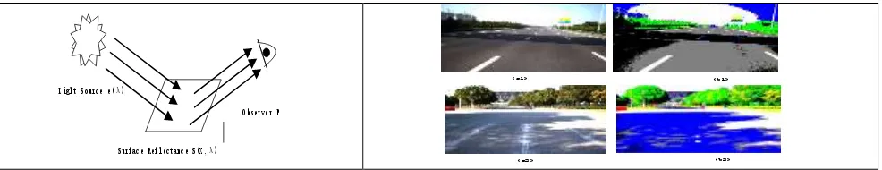
c   R G B is the camera sensitivity function [26]. As shown in figure 3, Weijer et al.

[4] proposed an edge-based color constancy algorithm by incorporating higher-order derivatives of an image based on grey-edge hypothesis, which assumes that the average of reflectance differences in a scene is achromatic. By introducing Minkowski-norm and Gauss filter; it becomes

1

, ,

( )

( ( ) )

n

p p n p

n

f X

dx ke

X





 _





where ( , , )T

f  R G B represents the image color, X is the spatial coordinate again, and f( )x f G

is the convolution of the image with a Gaussian filter G with a standard deviation .

n

n

X

 

 is an n-order derivative for f p is the Minkowski-norm. Equation (9) is obviously a general framework that can reformulate many existing algorithms by changing the parameters n p, , reflect the assumptions of the relationship between illumination and image colors. A. Gijisenij et al. points out that the different image texture feature is suitable to different color constancy algorithms. So the color constancy algorithm can be used as a global image features extraction method. The algorithm candidate set 0,1,0 0, ,0 0,1,2 1,1,1 2,1,1

{ , , , , }

M  e e  e e e did well in the study of constancy, and development mature in the research of feature fusion.

Light Source e(λ)

Surface Reflectance S(X,λ)

Observer P 002.png

（a1） （b1）

（b2） （a2）

Von Kries

Because the surface reflectivity and the color of the light source are unknown, this is an ill-posed problem and cannot be solved without additional constraints or assumptions [7]. Research on color constancy computation the goal is to eliminate the influence of scene illumination. The image of the unknown imagef_e illuminant color value (Re,Ge,Be), which will deviate from the actual ambient light source, is multiplied by the diagonal matrix D to process the imagef_a color value (Ra,Ga,Ba) of the

standard white illuminant source [15],[16]. Its expression is shown in 10

            e a e a e a e a B B G G R R f f f 0 0 0 0 0 0 D e (10)

Diagonal matrix D is a transformation coefficient matrix. J. von Kries et al. [14] proposed a von Kries model (also known as diagonal model); respectively, the RGB three channel color values were corrected.

Multiple Illuminants

Once local illuminant estimates are obtained per super-pixel, the local information can be combined as follows for the final computation of the number and color of the dominant illuminants in the scene. An example of this process is shown in Figure 4. The details of each of the aforementioned steps are provided in the following subsections. Group local estimates into regions with similar illuminant color. The downscaling suppresses a large amount of relatively small noisy regions. The same color in the scene area is considered to be the same kind of light source. In this relatively large connection area that considered only a light value and obtain a new estimate per illuminant region [17]. The area is used to estimate illuminant and color correction, the purpose is to multi-illuminant translate into a single illuminant problems.

Experiments

In this paper, the test is with the SFU subset [30].The SFU subset contains 15 groups of images taken in different places. Following the scheme of Gijsenij et al.[31],to ensure that the training and testing subsets are truly distinct, the 1,135 images are partitioned into 15 subsets based on geographical location. One subset is used for testing and the other 14 are used for training. This procedure is repeated 15 times with different test set selection.

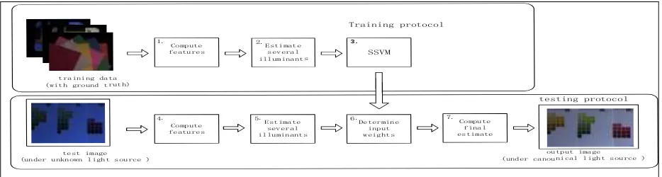
Estimate several illuminants Compute features Estimate several illuminants Compute features 1. 2. 5. 4. Determine input weights Compute final estimate 6. 7. Training protocol testing protocol training data

(with ground truth)

test image (under unknown light source )

output image (under canounical light source ) SSVM

3.

Figure 5. Illuminant color estimation process.

Error Measures

2 2

( ) ( )

i di st a e a e

E_  r  r  g  g (11)

For the distance error, we also compute the root mean square (RMS), mean, and median errors over a set of N test images. It has been argued that the median is the most appropriate metric for evaluating color constancy [24]. The standard RMS is defined as:

2 1

1 N

di st i di st

i

RMS E

N  





The second error measure is the angular error between the chromaticity 3-vectors when the b-chromaticity component is included. Given r andg, b = 1 – r – g. Thus, we can view the real illumination and estimated illumination as two <r,g,b> vectors in 3D chromaticity space and calculate the angle between them. The angular error represented in degrees is:

We also compute the RMS, mean, and median angular error over a set of images. Even if the median angular error for one method is less than for another, the difference may not be statistically significant. To evaluate whether a difference is significant, we use the Wilcoxon signed-rank test [24]. In the experiments, the error rate for accepting or rejecting null hypothesis is always set to 0.01.

Experimental Result Analysis

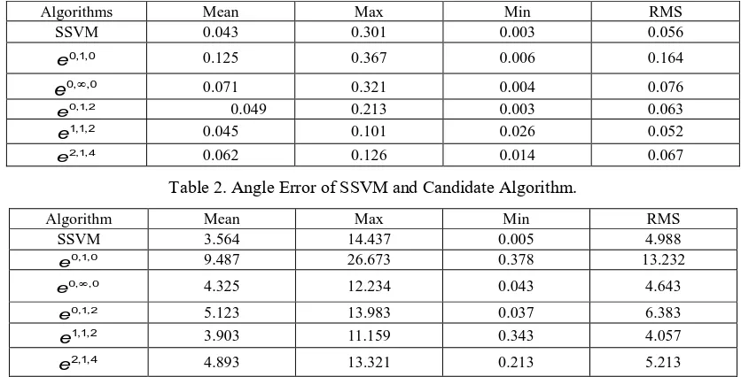
SSVM algorithm is used to fuse the multi-features extracted from the image, which to evaluate the image of the scene illuminant. In the SSVM algorithm, RBF kernel function is chosen to deal with the complex nonlinear problem of color constancy. Based on the realization of k-fold cross-validation, we find the optimal penalty parameter c and the parameter sig2 in RBF kernel function. All the training samples are divided into k groups, then k-1 group is selected as the training sample, and k group is used as the test [28]. There are 1,135 images in the dataset, of which 900 are used to build the learning model of the SSVM algorithm, and the remaining 235 are used to test the effect of color constancy. The error analysis is shown in Table 1 and Table 2:

Table 1. Chromaticity error of SSVM and candidate algorithms.

Algorithms Mean Max Min RMS

SSVM 0.043 0.301 0.003 0.056

0,1,0

e 0.125 0.367 0.006 0.164

0, ,0

e  0.071 0.321 0.004 0.076

0,1,2

e 0.049 0.213 0.003 0.063

1,1,2

e 0.045 0.101 0.026 0.052

2,1,4

e 0.062 0.126 0.014 0.067

Table 2. Angle Error of SSVM and Candidate Algorithm.

Algorithm Mean Max Min RMS

SSVM 3.564 14.437 0.005 4.988

0,1,0

e 9.487 26.673 0.378 13.232

0, ,0

e  4.325 12.234 0.043 4.643

0,1,2

e 5.123 13.983 0.037 6.383

1,1,2

e 3.903 11.159 0.343 4.057

2,1,4

e 4.893 13.321 0.213 5.213

From Table 1 on the 11 kinds of illuminant conditions, the chromaticity difference analysis shows that the SSVM fusion algorithm to obtain the smallest error, but with the algorithm _e1,1,2 _results

1 , ,

2 2 2 2 2 2

( , ) ( , ) 2π

[ ]

360

a a a e e e

i angul ar

a a a e e e

r g b r g b

E COS

r g b r g b



  

are similar. While the results of algorithm _e0,1,2 _and 2,1,4

e are similar, and the constancy of the effect is also very good. The effect of the gray world algorithm 0,1, 0

e is the worst, and the error is two times higher than that of the SSVM algorithm. The results show that the fusion algorithm can get closer to the true image of illuminant, and the gray world algorithm for measuring image due to the dark, unable to meet the corresponding assumptions and the constancy of poor effect. The error value of SSVM is 3. 564 degrees from the angle of Table 2, the effect better than the 1,1,2

e algorithm. The gray world algorithm results is the worst, the other three algorithms were similar. The constancy effect than fusion algorithm almost. In general, the fusion algorithm of error analysis is SSVM to obtain the color value of the light source which is close to the real scene.

Conclusion

Many previous methods of estimating the aromaticity of the scene illumination have been based in one way or another on statistics of the RGB colors arising in an image, independent of their spatial location or frequency of occurrence in the image [27]. Structured Support Vector Machine is a relatively new tool developed primarily for machine learning that can be applied in a similar way. We have tried it here, with good results, to the problem of learning the association between color histograms and illumination chromaticity. Under almost the same experimentation conditions as those used by Barnard [29], tests of the shades-of-grey, neural-network, color-by-correlation, Max RGB, and Gray-world methods, show that SSVM performance generally is comparable to or better than these other methods.

Acknowledgement

This paper is supported by the following projects：The National Natural Science Foundation of China (No. 61372148,No.61571045); Beijing Natural Science Foundation (No.4152016, No.4152018); Beijing Advanced Innovation Center for Imaging Technology (BAICIT-2016002); The National Key Technology R&D Program (2014BAK08B02，2015BAH55F03).

References

[1] Buchsbaum G. A spatial processor model for object colour perception [J]. Journal of the Franklin Institute, 1980, 310(1):1-26.

[2] Van d W J, Gevers T, Gijsenij A. Edge-Based Color Constancy [J]. IEEE Transactions on Image Processing A Publication of the IEEE Signal Processing Society, 2007, 16(9):2207-14.

[3] Finlayson G D, Trezzi E. Shades of Gray and Colour Constancy[C]// The Twelfth Color Imaging Conference: Color Science and Engineering Systems, Technologies, Applications, CIC 2004, November 9, 2004, Scottsdale, Arizona, USA. 2004:37-41.

[4] Gijsenij A, Gevers T, Van d W J. Improving color constancy by photometric edge weighting.[J]. Middle East Journal of Scientific Research, 2014, 34(5):1-1.

[5] J. van de Weijer, C. Schmid. Blur robust and color constant image description. In: Proc. of Int. Conf. on Image Processing (ICIP), 2006: 993-996.

[6] Buchsbaum G. A spatial processor model for object colour perception [J]. Journal of the Franklin Institute, 1980, 310(1):1-26.

[7] Land E H. The retinex theory of color vision. [J]. Scientific American, 1977, 237(6):108-28.

[9] Forsyth D A. A novel algorithm for color constancy [J]. International Journal of Computer Vision, 1990, 5(1):5-36.

[10] D. H. Brainard and W. T. Freeman. Bayesian Color Constancy [J]. Journal of the Optical Society of America A (Optics, Image Science and Vision). 1997, 14(7): 1393-1411.

[11] Li B, Xiong W, Hu W, et al. Evaluating Combinational Illumination Estimation Methods on Real-World Images.[J]. IEEE Transactions on Image Processing, 2014, 23(3):1194-209.

[12] Peter V. Gehler, Carsten Rother, Andrew Blake, Toby Sharp and Tom Minka. Bayesian Color Constancy Revisited. In: Proc. Of IEEE Int. Conf. on Computer Vision and Pattern Recognition (CVPR), 2008:1-8.

[13] Li B, Xiong W, Xu D, et al. A supervised combination strategy for illumination chromaticity estimation[J]. Acm Transactions on Applied Perception, 2010, 8(1):885-900.

[14] Beigpour S, Riess C, Weijer J V D, et al. Multi-Illuminant Estimation With Conditional Random Fields[J]. IEEE Transactions on Image Processing A Publication of the IEEE Signal Processing Society, 2014, 23(1):83-96.

[15] J. V. Weijer, T. Gevers, A. Gijsenij. Edge-Based Color Constancy. IEEE Trans, on Image Processing, 2007, 16(9): 2207-2214.

[16] Riess C, Eibenberger E, Angelopoulou E. Illuminant color estimation for real-world mixed-illuminant scenes[C]// IEEE International Conference on Computer Vision Workshops. IEEE, 2011:782-789.

[17] Tezaur R. Automatic illuminant estimation and white balance adjustment based on color gamut unions: US, US8860838[P]. 2014.

[18] W. Xiong, B. Funt. Estimating Illumination Chromaticity via Support Vector Regression. Journal of Imaging Science and Technology, 2006, 50(4): 341-348.

[19] Tsochantaridis I, Joachims T, Hofmann T, et al. Large Margin Methods for Structured and Interdependent Output Variables[J]. Journal of Machine Learning Research, 2005, 6(2):1453-1484.

[20] Sugumaran V, Sabareesh G R, Ramachandran K I. Fault diagnostics of roller bearing using kernel based neighborhood score multi-class support vector machine[J]. Expert Systems with Applications, 2008, 34(4):3090-3098.

[21] Joachims T, Finley T, Yu C N J. Cutting-plane training of structural SVMs[J]. Machine Learning, 2009, 77(1):27-59.

[22] Yue Y, Joachims T. Predicting diverse subsets using structural SVMs.[C]// International Conference, Helsinki, Finland, June. 2009:1224-1231. Li L, Zhou K, Xue G R, et al. Video Summarization via Transferrable Structured Learning[C]// International Conference on World Wide Web, WWW 2011, Hyderabad, India, March 28 - April. 2011:287-296.

[23] Park K J. Discrimination of outer membrane proteins using support vector machines [J]. Bioinformatics, 2005, 21(23):4223-9.

[24] Ward J J, Mcguffin L J, Buxton B F, et al. Secondary structure prediction with support vector machines [J]. Bioinformatics, 2003, 19(13):1650-5.

[25] Tian Y, Ju X, Qi Z. Efficient sparse nonparallel support vector machines for classification [J]. Neural Computing & Applications, 2014, 24(5):1089-1099.

[27] Bleier M, Riess C, Beigpour S, et al. Color constancy and non-uniform illumination: Can existing algorithms work?[C]// IEEE International Conference on Computer Vision Workshops, ICCV 2011 Workshops, Barcelona, Spain, November. 2011:774-781.

[28] Mosny M, Funt B. Reducing Worst-Case Illumination Estimates for Better Automatic White Balance[C]// Color and Imaging Conference. 2012:52-56(5).

[29] V. Cardei, B. Funt, K. Barnard, Estimating the Scene Illumination Chromaticity Using a Neural Network. Journal of the Optical Society of America A, 2002,19(12):2374-2386.

[30] Bianco S, Ciocca G, Cusano C, et al. Improving Color Constancy Using Indoor–Outdoor Image Classification[J]. IEEE Transactions on Image Processing, 2008, 17(12):2381-2392.