Munich Personal RePEc Archive
Bootstrap prediction intervals for
threshold autoregressive models
Jing, Li
South Dakota State University
January 2009
Online at
https://mpra.ub.uni-muenchen.de/13086/
Bootstrap Prediction Intervals For Threshold Autoregressive
Models
Jing Li
∗Department of Economics
South Dakota State University
Abstract
This paper examines the performance of prediction intervals based on bootstrap for
threshold autoregressive models. We consider four bootstrap methods to account for
the variability of estimates, correct the small-sample bias of autoregressive coefficients
and allow for heterogeneous errors. Simulation shows that (1) accounting for the
sam-pling variability of estimated threshold values is necessary despite super-consistency,
(2) bias-correction leads to better prediction intervals under certain circumstances,
and (3) two-sample bootstrap can improve long term forecast when errors are
regime-dependent.
Keywords: Bootstrap; Interval Forecasting; Threshold Autoregressive Models; Time
Series; Simulation
∗Department of Economics, Scobey Hall, Box 504, South Dakota State University, Brookings, SD 57007.
Introduction
Constructing prediction intervals is an important topic in forecasting time series. One can
construct classical prediction intervals (CPI) for an autoregression (AR) using the
Box-Jenkins method, see Granger and Newbold (1986) for instance. In practice two factors may
worsen the finite-sample performance of CPI. First, the distribution of prediction errors
may be non-normal. Second, CPI may fail to take into account the sampling variability of
estimated autoregressive coefficients. The second factor directly causes the under-nominal
coverage of CPI found in previous studies such as Thombs and Schucany (1990) and Kim
(2001).
The non-normal prediction error plays a more important role for the threshold
autore-gressive (TAR) model developed by Tong (1983). All estimated autoreautore-gressive coefficients
in TAR models are functions of the estimated threshold value, which is well known to follow
a nonstandard distribution. Therefore prediction errors of TAR models (calculated as the
difference between true future values and predicted values) follow nonstandard distributions
by construction.
Given these limitations of CPI, bootstrap prediction intervals (BPI) for TAR models are
widely used by practitioners, though the performance of BPI has not been systematically
investigated. This paper is intended to fill the gap. In particular, four methods of
construct-ing BPI are considered. The first issue is unique to TAR models, and is concerned with
the estimated threshold value. Chan (1993) proves that the threshold value estimated by
grid-searching is super-consistent. That means for some problems of statistical inference we
can treat the estimated threshold value as the true value and ignores its sampling variability.
In this paper we investigate whether it is worthwhile to account for that sampling variability
when constructing BPI. The second issue is related to the small-sample bias of estimated
autoregressive coefficients. Following Kilian (1998) and Kim (2001) we adopt the
The last issue is unique to TAR models with regime-dependent errors, for which
construct-ing BPI belongs to the “two-sample problem” in the terminology of Efron and Tibshirani
(1993). Existing literature typically downplays this problem. But we propose a method
of bootstrapping separately the residuals in each regime (called two-sample bootstrap
here-after), instead of bootstrapping the pooled residuals. In this paper we do not consider the
percentile-t method since it is theoretically difficult to compute the asymptotic standard
error and its bootstrap counterpart (ˆσck(h) and ˆσ∗
k(h) in Kim (2001)) for TAR models.
BPI for linear autoregressive models is studied by several authors. Among others, Thombs
and Schucany (1990) generate bootstrap replicates based on backward AR models. Kim
(2001) and Kim (2002) apply the bootstrap-after-bootstrap method of Kilian (1998) to
cor-rect the bias of autoregressive coefficients. Masarotto (1990) and Grigoletto (1998) build
BPI based on forward AR models. Kim (1999) and Kim (2004) consider BPI for vector
autoregressions.
In this paper, the performance of four BPIs for the nonlinear TAR model is compared
by extensive simulation. Special attention is paid to scrutinizing the effects of (I) magnitude
of varying coefficients across regimes, (II) the number of observations subject to
regime-switching, (III) the degree of heterogeneity in errors and (IV) the possible non-stationarity.
(I) (II) and (III) have not been discussed in above papers since they are irrelevant to linear
models.
The remainder of the paper is organized as follows. Section 2 specifies the TAR model.
A simple simulation is used to highlight the nonstandard distribution of predicted values
of TAR models. Three methods of constructing BPI for TAR models with regime-invariant
errors are provided in Section 3. Section 4 constructs BPI for TAR models with
regime-varying errors. Simulation is conducted in Section 5, and Section 6 concludes. Without
TAR Models
The observed data are (y1, . . . , yn),with initial conditions (y0, y−1, . . . , y−p+1). A two-regime
self-exciting threshold autoregressive (SETAR) model of order pis specified as
yt= Ã
β10+
p X
j=1
β1jyt−j !
1(yt−1 > γ) +
Ã
β20+
p X
j=1
β2jyt−j !
1(yt−1 ≤γ) +et, (1)
where et is the error with a common distribution function Fe. We do not assume a specific
parametric form of Fe. However, we do assume et ∼ iid(0, σ2) to facilitate the residual
bootstrap. The lag order p can be chosen based on information criteria such as AIC and
BIC. After fitting (1) one may check whether residuals are serially uncorrelated to ensure
bootstrap works properly.
The threshold value is denoted byγ, and 1(.) denotes the indicator function that equals
one if the event inside the parentheses is true and zero otherwise. In regime one yt−1 is
greater than γ, and is less than or equal to γ in regime two. At a given lag j, model (1)
allows for different autoregressive coefficients across regimes. The threshold effect exists if
β1j 6=β2j for some j. A formal test for the threshold effect is developed in Chan (1990).
The unknown threshold value can be estimated by grid-searching as follows. For given
γ we define the indicator and fit model (1) by OLS. We do this for a range of γ ∈ [γl, γu],
where the lower and upper searching bounds are the τth and (100−τ)th percentiles of the
empirical distribution of yt−1. In this paper τ = 15 is used throughout. The value of γ
minimizing the residual sum of squares (RSS) is the estimated threshold value:
ˆ
γ =argminγ∈[γl,γu]RSS(γ). (2)
Chan (1993) shows that the estimated threshold value (2) is super-consistent, thereby
example, an exogenous variable can serve as the threshold variable entering the indicator.
A three-regime or band TAR model can be specified by defining 1(yt−1 > γ2) for regime 1,
1(γ1 ≤ yt−1 ≤ γ2) for regime 2 and 1(yt−1 < γ1) for regime 3. In addition, one can specify
the indicator as 1(yt−d > γ) with unknown d. Then grid-searching γ can be nested into the
search for the number of regimes and d. For expositional purpose, the following discussions
are based on the basic model (1) (so that TAR is synonymous with SETAR in this paper).
After estimating ˆγ by (2) and fitting model (1) with ˆγ, compute residuals as
ˆ
et=yt− Ã
ˆ β10+
p X
j=1
ˆ β1jyt−j
!
1(yt−1 >γˆ)−
Ã
ˆ β20+
p X
j=1
ˆ β2jyt−j
!
1(yt−1 ≤γˆ), (3)
where ˆβij denotes the least squares estimate of the coefficient. By construction the residual
is centered at zero. We do not re-scale the residual since preliminary simulation shows little
effect of re-scaling. Leth≥1 denote the forecast horizon. Then the h-step-ahead predicted
value conditional on the last p observations of yt can be computed as
ˆ yt+h =
Ã
ˆ β10+
p X
j=1
ˆ
β1jyˆt+h−j !
1(ˆyt+h−1 >ˆγ) +
Ã
ˆ β20+
p X
j=1
ˆ
β2jyˆt+h−j !
1(ˆyt+h−1 ≤γˆ), (4)
where ˆyt =yt,(t=n, n−1, . . . , n−p+ 1).
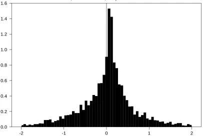
The nonstandard distribution of estimated threshold value is established in Hansen
(2000). The predicted values of TAR models by construction are linear combinations of
esti-mated autoregressive coefficients, which are themselves functions of the estiesti-mated threshold
value. Thus, it is not surprising that the predicted values (and prediction errors) follow
nonstandard distributions. To see this, we generate 5000 1-step-ahead predicted values from
the TAR model: yt = 0.2yt−11(yt−1 > 0) + 0.8yt−11(yt−1 ≤ 0) + et,(t = 1, . . . , n), where
n= 60, et∼iidn(0,1), y0 = 0. The standard normal erroret is used to highlight the role of
displays the histogram of standardized ˆyt+1and corresponding statistics. First the significant
skewness and kurtosis cast doubt on normality. Then the Jarque-Bera test of Jarque and
Bera (1987) formally rejects normality for standardized ˆyt+1 at 0.01 level. This simulation
demonstrates that the assumption of normal prediction errors is invalid for TAR models.
One-Sample Bootstrap Prediction Intervals for TAR Models
Given the nonstandard distribution of prediction errors, we consider bootstrap prediction
intervals for TAR models. The point is to use bootstrap to “automatically” account for the
variability of estimated parameters and non-normality of prediction errors. Four bootstrap
methods are proposed depending on whether accounting for the variability of estimated
threshold values, whether correcting for the bias of autoregressive coefficient and whether
generalizing model (1) by heterogeneous errors.
Chan (1993) shows that ˆγ in (2) is n-consistent. This super-consistency implies that it
is plausible to construct prediction intervals by ignoring the variability of ˆγ. Method 1 uses
this idea and consists of the following steps.
Method 1
Step 1-1. Let Feˆ denote the empirical cdf of ˆet computed by (3). Then use ˆγ, βˆij, and
generate recursively the bootstrap replicate of yt (denoted byyt∗) as
y∗
t =yt, t= 1, . . . , p,
y∗
t = Ã
ˆ β10+
p X
j=1
ˆ β1jyt∗−j
!
1(y∗
t−1 >ˆγ) +
Ã
ˆ β20+
p X
j=1
ˆ β2jy∗t−j
!
1(y∗
t−1 ≤ˆγ) +e
∗
t,(t > p)
where e∗
t is a random draw fromFˆe (ie., a draw from {eˆt}nt=p+1 with replacement).
Step 1-2. Re-estimate Model (1) usingy∗
t and ˆγ,and obtain bootstrap coefficients ˆβ
∗
compute a bootstrap h-step-ahead future value (denoted by ˆy∗
t+h):
ˆ y∗
t =yt, t=n, n−1, . . . , n−p+ 1,
ˆ y∗
t+h = Ã ˆ β∗ 10+ p X j=1 ˆ β∗
1jyˆ
∗
t+h−j !
1(ˆy∗
t+h−1 >γˆ) +
à ˆ β∗ 20+ p X j=1 ˆ β∗
2jyˆ
∗
t+h−j !
1(ˆy∗
t+h−1 ≤γˆ) +e
∗
t+h,
where e∗
t+h is a random draw from Feˆ.
Step 1-3. Repeat Step 1-1 and 1-2 B times and obtain a series of bootstrap future values
©
ˆ y∗
t+h(i) ªB
i=1, where i indexes resampling. The Method-1 h-step-ahead BPI at 0.95
nominal level is given by
BPI1= [ˆyt.025+h,yˆ.t975+h] (5)
where ˆy.025
t+h and ˆyt.975+h are the 2.5th and 97.5th percentiles of the empirical cdf of
©
ˆ y∗
t+h(i) ªB
i=1.
First notice that in Step 1-1 we generate the bootstrap replicate in the forward model. The
backward representation used by Thombs and Schucany (1990), Kim (2001) and others is
unavailable for TAR models since it is impossible to invert the lag polynomial augmented
with indicators. Second, following Efron and Tibshirani (1986) we use the firstpobservations
of observed series as initial values for bootstrap replicates. Alternatively one may use any
block ofpobservations ofyt.In Step 1-2 we compute bootstrap forecasts always using the last
pobservations of observed series. The importance of this conditionality on lastpobservations
is stressed in Maekawa (1987), Chatfield (1993) and Kim (2001). Note Method 1 accounts
for the sampling variability of ˆβij but ignores its small-sample bias shown by Shaman and
Stine (1988). That bias is corrected by Method 2 as follows.
Method 2
Step 2-2. Re-estimate Model (1) using y∗
t and ˆγ, and obtain bootstrap coefficients ˆβ
∗
ij.
Repeat this process C times, and get a series of bootstrap coefficients nβˆ∗
ij(k) oC
k=1,
wherek indexes resampling. Compute the bias-corrected autoregressive coefficients as
ˆ
βijc = 2 ˆβij −C−1
C X
k=1
ˆ β∗
ij(k),(i= 1,2, j = 0,1, . . . , p). (6)
Step 2-3. Use ˆβc
ij to generate the bias-corrected bootstrap replicate asyc
∗
t =yt, t = 1, . . . , p,
and
yc∗
t = Ã
ˆ β10c +
p X
j=1
ˆ β1cjyc∗
t−j !
1(yc∗
t−1 >γˆ) +
Ã
ˆ β20c +
p X
j=1
ˆ β2cjyc∗
t−j !
1(yc∗
t−1 ≤γˆ) +e
∗
t.(t > p),
where e∗
t is a random draw fromFˆe.
Step 2-4. Re-estimate Model (1) usingyc∗
t and ˆγ,and obtain coefficients ˆβc
∗
ij.Then compute
a bias-corrected bootstrap future value as ˆyc∗
t =yt, t =n, n−1, . . . , n−p+ 1,and
ˆ yc∗
t+h = Ã
ˆ βc∗
10+
p X
j=1
ˆ βc∗
1jyˆ
∗
t+h−j !
1(ˆyc∗
t+h−1 >γˆ)+
Ã
ˆ βc∗
20+
p X
j=1
ˆ βc∗
2jyˆ c∗
t+h−j !
1(ˆyc∗
t+h−1 ≤γˆ)+e ∗
t+h,
where e∗
t+h is a random draw from Feˆ.
Step 2-5. Repeat Step 2-1, 2-2, 2-3 and 2-4 B times and obtain a series of bias-corrected
bootstrap future values©
ˆ yc∗
t+h(i) ªB
i=1. The Method-2 h-step-ahead BPI is given by
BPI2= [ˆy.t025+hc,yˆ.t975+hc] (7)
where ˆy.025c
t+h and ˆyt.975+hc are the 2.5th and 97.5th percentiles of the empirical cdf of
©
ˆ yc∗
t+h(i) ªB
Basically, Step 2-2 calculates the bias-corrected autoregressive coefficients following Kilian
(1998) and Kim (2001). Then Step 2-3 generates bootstrap replicates using the bias-corrected
coefficients. Notice that Steps 2-3 and 2-4 resample original residuals. Alternatively, one
may compute new residuals by (3) using bias-corrected coefficients (6), and redo Step 2-3
and 2-4 using random draws from new residuals.
Method 1 and Method 2 both ignore the variability of the estimated threshold value since
ˆ
γ is not re-estimated using bootstrap replicates. Method 3, on the other hand, explicitly
takes into account the variability of ˆγ. The algorithm of Method 3 is as follows.
Method 3
Step 3-1. The same as Step 1-1.
Step 3-2. use y∗
t and estimate the bootstrap threshold value ˆγ
∗
from (2). Then re-estimate
Model (1) using y∗
t and ˆγ
∗
, and obtain bootstrap coefficients ˆβijγ∗. Next compute a
bootstrap h-step-ahead future value ˆytγ∗ =yt, t =n, n−1, . . . , n−p+ 1,and
ˆ yγ∗
t+h = Ã
ˆ βγ∗
10 +
p X
j=1
ˆ βγ∗
1jyˆ γ∗
t+h−j !
1(ˆyγ∗
t+h−1 >γˆ
∗
)+
Ã
ˆ βγ∗
20 +
p X
j=1
ˆ βγ∗
2jyˆ γ∗
t+h−j !
1(ˆyγ∗
t+h−1 ≤γˆ
∗
)+e∗
t+h,
where e∗
t+h is a random draw from Feˆ.
Step 3-3. Repeat Step 3-1 and 3-2 B times and obtain a series of bootstrap future values
©
ˆ yγ∗
t+h(i) ªB
i=1. The Method-3 h-step-ahead BPI is given by
BPI3= [ˆyt.025+hγ,yˆ.t975+hγ] (8)
where ˆy.t025+hγ and ˆyt.975+hγ are the 2.5th and 97.5th percentiles of the empirical cdf of
©
ˆ yγ∗
t+h(i) ªB
Note that the threshold value is re-estimated in Step 3-2. To ease computation Method 3
does not correct the bias of autoregressive coefficients, though it is straightforward to add the
bias-correcting procedure. Bias-correcting ˆγ is unnecessary because of its super consistency.
Two-Sample Bootstrap Prediction Intervals of TAR Models
Model (1) assumes a regime-invariant distribution function foret.Then bootstrapping model (1)
belongs to what is called “one-sample problems” in Efron and Tibshirani (1993). More
gen-erally, we can allow for regime-dependent errors and write the generalized model as
yt= Ã
β10+
p X
j=1
β1jyt−j+e1t !
1(yt−1 > γ) +
Ã
β20+
p X
j=1
β2jyt−j+e2t !
1(yt−1 ≤γ), (9)
where e1t ∼ iid(0, σ21) and e2t ∼ iid(0, σ22). Let Fe1 and Fe2 be the distribution functions
for e1t and e2t. Then Model (9) makes it possible Fe1 6=Fe2. Method 4 explicitly takes into
account this possible heterogeneity by bootstrapping separately two samples of residuals.
Method 4
Step 4-1. Estimate ˆγ by (2) and define regime 1 and 2 accordingly. Then fit Model (1)
using ˆγ and compute the residual ˆetby (3). Collect observations of{eˆt}nt=p+1 in regime
1 as the series of{eˆ1t}nt=11 ,and in regime 2 {eˆ2t}nt=12 ,where n1 +n2 = n−p.
Step 4-2. Let Feˆ1 and Fˆe2 denote the empirical cdfs of ˆe1t and ˆe2t computed in Step 4-1.
Then generate the bootstrap replicate of yt as ytt∗ =yt, t= 1, . . . , p, and
yt∗
t = Ã
ˆ β10+
p X
j=1
ˆ
β1jytt−∗j +e
∗
1t !
1(yt∗
t−1 >γˆ)+
Ã
ˆ β20+
p X
j=1
ˆ
β2jytt∗−j +e
∗
2t !
1(yt∗
t−1 ≤γˆ),(t > p)
where e∗
1t and e
∗
2t are random draws from Fˆe1 and Feˆ2 respectively.
Step 4-3. Re-estimate Model (1) usingyt∗
t and ˆγ,and obtain bootstrap coefficients ˆβt
∗
compute a bootstrap h-step-ahead future value: ˆyt∗
t =yt, t =n, n−1, . . . , n−p+ 1,
ˆ yt∗
t+h = Ã
ˆ βt∗
10+
p X
j=1
ˆ βt∗
1jyˆ t∗
t+h−j+e
∗
1t+h !
1(ˆyt∗
t+h−1 >ˆγ)+
Ã
ˆ βt∗
20+
p X
j=1
ˆ βt∗
2jyˆt
∗
t+h−j +e
∗
2t+h !
1(ˆyt∗
t+h−1 ≤γˆ),
where e∗
1t+h and e
∗
2t+h are random draws fromFeˆ1 and Fˆe2 respectively.
Step 4-4. Repeat Step 4-2 and 4-3 B times and obtain a series of bootstrap future values
©
ˆ yt∗
t+h(i) ªB
i=1, where i indexes the number of resampling. The Method-4 h-step-ahead
BPI is given by
BPI4= [ˆy.025two
t+h ,yˆ .975two
t+h ] (10)
where ˆy.025two
t+h and ˆy.975
two
t+h are the 2.5th and 97.5th percentiles of the empirical cdf of
©
ˆ yt∗
t+h(i) ªB
i=1.
It is easy to modify Method 4 to account for the variability of ˆγ and correct the bias of
autoregressive coefficients.
Simulation
This section compares the performance of BPIs by Monte Carlo simulation. Following
Thombs and Schucany (1990), the criterion of comparison is the average coverage rate
com-puted as
m−1
m X
i=1
1 (yt+h ∈PI), (11)
where m = 100 for each replication and PI denotes BPI1 (5), BPI2 (7), BPI3 (8) and
BPI4 (10). The forecast horizon h ranges from 1 to 8 (no qualitative changes in simulation
results are found when h ranges from 1 to 12, or larger value). The number of Monte Carlo
Method 3 and Method 4. For Method 2, the number of resampling isC = 200 for Step 2-2,
and B = 999 for Step 2-5. The nominal coverage rate is 0.95. The method that produces
prediction intervals with the average coverage rate closest to 0.95 is deemed the best method.
We first consider the data generating process with homogeneous (regime-invariant) errors:
yt=c1yt−11(yt−1 > γ) +c2yt−11(yt−1 ≤γ) +et,(t= 1, . . . , n), (12)
where the threshold effect (or magnitude of regime-switching) is measured by coefficientsc1
andc2.The number of observations subject to regime switching is controlled byγ.Figures 2,
3, 4, 5 plot the average coverage rates of BPI1, BPI2 and BPI3 against the forecast horizon
h(this is a “one-sample” problem so we ignore BPI4). A note about the key in those figures:
the number after the underlining sign indexes graphs. For example, in Figure 2 BPI1 1
denotes the coverage rate of BPI1 in the first graph, and BPI3 2 the coverage rate of BPI3
in the second graph, and etc.
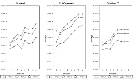
First we let c1 = 0.2, c2 = 0.8, γ = 0.0, n = 60. Figure 2 shows the effect of various
distributions of et on the coverage rate. We simulate errors using the standard normal
distribution, the Student-T distribution with 5 degrees of freedom, and the chi-squared
distribution with 4 degree of freedom. The Student-T and chi-squared distributions are fat
tailed and skewed, respectively. Following Thombs and Schucany (1990) the non-normal
errors are standardized prior to simulation.
We have four findings from Figure 2. First we see no severe distortion in coverage rates:
the coverage rates of BPIs are bounded between 0.94 and 0.96 in most cases. This means
bootstrap prediction intervals work generally well with various error distributions. Second,
the coverage rate of BPI1 is always the lowest one among the three methods. This fact
comes as no surprise since BPI1 ignores the variability of estimated threshold value, ˆγ. On
The wide BPI2 is consistent with Efron and Tibshirani (1993), which point out that more
variability is introduced by bias-corrected statistics. In this case BPI2 is wider than BPI1
and BPI3 by using bias-corrected autoregressive coefficients. By accounting for variability
of ˆγ but without correcting the autoregressive bias, BPI3 yields the coverage in the middle.
For practitioners the lesson is that BPI2 and BPI3 may be more conservative than BPI1 in
terms of coverage rates. The third finding is, the skewed chi-squared distribution causes more
coverage-distortion (by shifting coverage lines up further) than the fat-tailed T distribution,
while the latter seems not to worsen BPIs very much. Finally, we find that as forecast horizon
hincreases, the coverage rates of all BPIs increase as well. Again this result is intuitive since
long-term forecast intrinsically involves more uncertainty than short-term forecast.
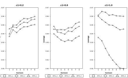
Figure 3 shows how regime-varying autoregressive coefficients affect coverage rates with
c1 = 0.2,0.8,1.0 and c2 = 0.8, γ = 0.0, n = 60, et ∼ iidn(0,1). The threshold effect is
present when c1 = 0.2 6= c2, and the results are basically the same as the left panel of
Figure 2. Threshold effect disappears (and a TAR model reduces to a linear AR model)
when c1 =c2 = 0.8. In this case, BPI1 and BPI3 suffer more under-nominal distortion than
BPI2. Hence it pays to apply the bias-correction procedure for the linear model, a result in
line with Kim (2001) and Kilian (1998). Something interesting happens when the data are
nonstationary in the regime withc1 = 1.0.Now BPI1 suffers severe under-nominal distortion,
with coverage rate declining monotonically with forecast horizon. BPI3 also has decreasing
coverage rate, though less severe than BPI1. The most stable (though slightly above nominal
level) coverage rate is produced by BPI2. Based on these findings, BPI2 is recommended
when the threshold effect is marginal or when data are possibly nonstationary.
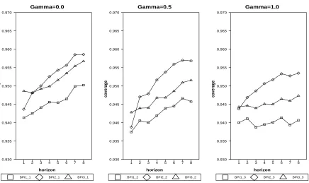
Figure 4 illustrates how the frequency of regime-switching affects coverage rates with
varyingγ andc1 = 0.2, c2 = 0.8, n = 60, et∼iidn(0,1). Asγ increases there is less and less
likelihood for regime-switching, and so more and more observations stay in one regime. In
performance of BPIs reflects this fact. Whenγ = 0.0,regime-switching occurs frequently and
the graph looks almost the same as the left panel of Figure 2. Whenγ = 1.0 regime-switching
becomes less likely (and the model is more like a linear model) and so the performance of
BPI2 is the best (without obvious under-nominal distortion) among the three methods. The
key message is that using BPI2 is a good idea where there is a small number of observations
subject to regime-switching.
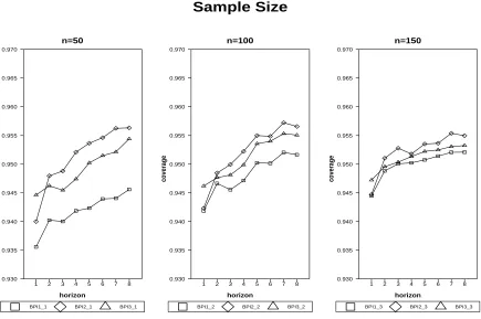
Figure 5 investigates the effect of sample sizes on coverage rates of BPIs, with n =
50,100,150 and c1 = 0.2, c2 = 0.8, γ = 0.0, et ∼ iidn(0,1). The increasing sample size is
seen to improve the coverage rate of all BPIs in two ways. First, asn rises the coverage rate
gets closer to the nominal level 0.95. Meanwhile, in large sample (n = 150) as h increases
the coverage rate increases more slowly than in the small sample (n = 50). For instance, as
h rises, BPI2 increases from 0.940 to above 0.955 when n = 50, while only increases from
0.945 to 0.955 when n= 150.
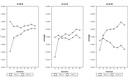
Next we consider the following TAR model with regime-dependent errors to investigate
the performance of BPI4:
yt = (c1yt−1+e1t)1(yt−1 > γ) + (c2yt−1 +e2t)1(yt−1 ≤γ),(t= 1, . . . , n), (13)
wheree1t∼iidn(0,1) and e2t∼iidn(0, s2),(s= 0.5,1.0,2.0) are (possibly) heteroskedastic
normal errors. Figure 6 only compares BPI1 and BPI4 with c1 = 0.2, c2 = 0.8, n = 60, γ =
0.0. We do not consider BPI2 and BPI3 here in order to focus on the difference between
“one-sample bootstrap” and “two-sample bootstrap.” The readers are reminded again that
it is straightforward to modify BPI4 so that variability of ˆγ and autoregressive bias can be
taken care of.
First of all, Figure 6 shows that both coverage rates of BPI1 and BPI4 are below the
it is shown that BPI4 has less under-nominal coverage distortion than BPI1 in most cases.
The exception is when s = 0.5, and when h is small. Nevertheless, it is constructive to
emphasize that BPI4 outperforms BPI1 when errors are homoskedastic (s= 1.0). So using
two-sample bootstrap loses nothing related to one-sample bootstrap when heteroskedasticity
is uncertain. In addition, by comparing the three panels of Figure 6, we see that the position
of the coverage line for BPI4 is relatively fixed, whereas the coverage line for BPI1 keeps
shifting down assrises. In light of this, loosely speaking, BPI4 is “heteroskedasticity-robust”
while BPI1 is not.
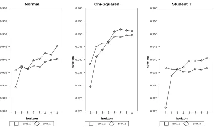
Figure 6 simulates e2t using standard normal distributions. Figure 7 instead simulates
e2t using the standard normal distribution, the Student-T distribution with 5 degrees of
freedom, and the chi-squared distribution with 4 degree of freedom. Now e1t and e2t are
heterogeneous, not just heteroskedastic. The findings from Figure 7 are more favorable to
BPI4 than Figure 6. With normal errors, the graph looks the same as the middle panel of
Figure 6. The chi-squared distribution tends to shift BPI4 up further (and cause less
under-nominal distortion) than BPI1, so does the T distribution. Overall, BPI4 outperforms BPI1
with various distributions, and the gain of using two-sample bootstrap increases with the
forecast horizon. For short term forecast, BPI1 may do better than BPI4 thanks to its
relatively simple algorithm.
To summarize, the key findings of simulation are following: (1) BPIs perform
gener-ally well. (2) It is necessary to account for the sampling variability of estimated threshold
value in finite sample even if it is asymptotically super-consistent. (3) The bias-correction in
the bootstrap-after-bootstrap procedure can generate better prediction intervals when the
threshold effect is minimal, when data are possibly nonstationary, and when the number of
observations subject to regime-switching is small. (4) Two-sample bootstrap, which
sepa-rately resamples residuals in two regimes, are necessary especially when errors are
Conclusion
This paper considers four methods of constructing bootstrap prediction intervals for TAR
models. The Method 1 is the simplest because it only accounts for the variability of estimated
autoregressive coefficients. Method 2 corrects the finite-sample bias of autoregressive
coeffi-cients. Method 3 takes into account the variability of estimated threshold values. Method
4 resamples residuals in separate regimes. The main finding of simulation is that
boot-strap prediction intervals perform generally well. Method 2 yields better prediction intervals
under certain circumstances. The two-sample bootstrap prediction intervals outperform
one-sample bootstrap prediction intervals when errors are regime-dependent and when forecast
References
Chan, K. S. (1990). Testing for threshold autoregression. The Annals of Statistics, 18,
1886–1894.
Chan, K. S. (1993). Consistency and limiting distribution of the least squares estimator of
a threshold autoregressive model. The Annals of Statistics, 21, 520–533.
Chatfield, C. (1993). Calculating interval forecasts. Journal of Business & Economic
Statis-tics, 11, 121–135.
Efron, B. and Tibshirani, R. J. (1986). Bootstrap methods for standard errors, confidence
intervals, and other measures of statistical accuracy. Statistical Science, 1, 54–75.
Efron, B. and Tibshirani, R. J. (1993). An Introduction to the Bootstrap. London: Chapman
and Hall.
Granger, C. and Newbold, P. (1986). Forecasting Economic Time Series. San Diego:
Aca-demic Press.
Grigoletto, M. (1998). Bootstrap prediction intervals for autoregressions: some alternatives.
International Journal of Forecasting, 14, 447–456.
Hansen, B. E. (2000). Sample splitting and threshold estimation. Econometrica, 68, 575–603.
Jarque, C. M. and Bera, A. K. (1987). A test for normality of observations and regression
residuals. International Statistical Review, 55, 163–172.
Kilian, L. (1998). Small sample confidence intervals for impulse response functions. The
Review of Economics and Statistics, 80, 218–230.
Kim, J. (1999). Asymptotic and bootstrap prediction regions for vector autoregression.
Kim, J. (2001). bootstrap-after-bootstrap prediction intervals for autoregressive models.
Journal of Business & Economic Statistics, 19, 117–128.
Kim, J. (2002). Bootstrap prediction intervals for autoregressive models of unknown or
infinite lag order. Journal of Forecasting, 21, 265–280.
Kim, J. (2004). Bias-corrected bootstrap prediction regions for vector autoregression.Journal
of Forecasting, 23, 141–154.
Maekawa, K. (1987). Finite sample properties of several predictors from an autoregressive
model. Econometric Theory, 3, 359–370.
Masarotto, G. (1990). bootstrap prediction intervals for autoregressions. International
Jour-nal of Forecasting, 6, 229–239.
Shaman, P. and Stine, R. A. (1988). The bias of autoregressive coefficient estimators.Journal
of the American Statistical Association, 83, 842–848.
Thombs, L. A. and Schucany, W. R. (1990). bootstrap prediction intervals for autoregression.
Journal of the American Statistical Association, 85, 486–492.
Tong, H. (1983). Threshold Models in Non-linear Time Series Analysis. New York:
Histogram of 1-Step-Ahead Predicted Value of TAR Models
Skewness=-0.69, Kurtosis=47.52, Jarque-Bera Test=64366.10
-2 -1 0 1 2
[image:20.595.82.488.106.384.2]0.0 0.2 0.4 0.6 0.8 1.0 1.2 1.4 1.6
Error Distribution
Normal
BPI1_1 BPI2_1 BPI3_1
horizon
coverage
1 2 3 4 5 6 7 8 0.930
0.935 0.940 0.945 0.950 0.955 0.960 0.965 0.970
Chi-Squared
BPI1_2 BPI2_2 BPI3_2
horizon
coverage
1 2 3 4 5 6 7 8 0.930
0.935 0.940 0.945 0.950 0.955 0.960 0.965 0.970
Student T
BPI1_3 BPI2_3 BPI3_3
horizon
coverage
1 2 3 4 5 6 7 8 0.930
[image:21.595.95.531.105.364.2]0.935 0.940 0.945 0.950 0.955 0.960 0.965 0.970
Threshold Effect
c1=0.2
BPI1_1 BPI2_1 BPI3_1
horizon
coverage
1 2 3 4 5 6 7 8 0.90
0.91 0.92 0.93 0.94 0.95 0.96 0.97
c1=0.8
BPI1_2 BPI2_2 BPI3_2
horizon
coverage
1 2 3 4 5 6 7 8 0.90
0.91 0.92 0.93 0.94 0.95 0.96 0.97
c1=1.0
BPI1_3 BPI2_3 BPI3_3
horizon
coverage
1 2 3 4 5 6 7 8 0.90
[image:22.595.94.531.98.364.2]0.91 0.92 0.93 0.94 0.95 0.96 0.97
Threshold Value
Gamma=0.0
BPI1_1 BPI2_1 BPI3_1
horizon
coverage
1 2 3 4 5 6 7 8 0.930
0.935 0.940 0.945 0.950 0.955 0.960 0.965 0.970
Gamma=0.5
BPI1_2 BPI2_2 BPI3_2
horizon
coverage
1 2 3 4 5 6 7 8 0.930
0.935 0.940 0.945 0.950 0.955 0.960 0.965 0.970
Gamma=1.0
BPI1_3 BPI2_3 BPI3_3
horizon
coverage
1 2 3 4 5 6 7 8 0.930
[image:23.595.95.531.106.365.2]0.935 0.940 0.945 0.950 0.955 0.960 0.965 0.970
Sample Size
n=50
BPI1_1 BPI2_1 BPI3_1
horizon
coverage
1 2 3 4 5 6 7 8 0.930
0.935 0.940 0.945 0.950 0.955 0.960 0.965 0.970
n=100
BPI1_2 BPI2_2 BPI3_2
horizon
coverage
1 2 3 4 5 6 7 8 0.930
0.935 0.940 0.945 0.950 0.955 0.960 0.965 0.970
n=150
BPI1_3 BPI2_3 BPI3_3
horizon
coverage
1 2 3 4 5 6 7 8 0.930
[image:24.595.96.531.79.368.2]0.935 0.940 0.945 0.950 0.955 0.960 0.965 0.970
Heteroskedasticity
s=0.5
BPI1_1 BPI4_1
horizon
coverage
1 2 3 4 5 6 7 8 0.910
0.915 0.920 0.925 0.930 0.935 0.940 0.945 0.950
s=1.0
BPI1_2 BPI4_2
horizon
coverage
1 2 3 4 5 6 7 8 0.910
0.915 0.920 0.925 0.930 0.935 0.940 0.945 0.950
s=2.0
BPI1_3 BPI4_3
horizon
coverage
1 2 3 4 5 6 7 8 0.910
[image:25.595.94.528.102.365.2]0.915 0.920 0.925 0.930 0.935 0.940 0.945 0.950
Heterogeneous Errors
Normal
BPI1_1 BPI4_1
horizon
coverage
1 2 3 4 5 6 7 8 0.920
0.925 0.930 0.935 0.940 0.945 0.950 0.955 0.960
Chi-Squared
BPI1_2 BPI4_2
horizon
coverage
1 2 3 4 5 6 7 8 0.920
0.925 0.930 0.935 0.940 0.945 0.950 0.955 0.960
Student T
BPI1_3 BPI4_3
horizon
coverage
1 2 3 4 5 6 7 8 0.920
[image:26.595.97.530.107.366.2]0.925 0.930 0.935 0.940 0.945 0.950 0.955 0.960