Markovian Bulk Service Queue Under
Accessibility Rules
S. Bharathidass,
PhD. Asst. Prof Department of StatisticsPeriyar E.V.R. College Trichy, Tamilnadu, India
ABSTRACT
A single server Markovian queue is considered. The arriving units are served in batches by using Accessibility and Non-Accessibility rules with varying service rates. The expressions for the steady state probabilities when the server is busy as well as idle are derived. The mean and variance for the number of units in the queue are obtained. The expected waiting time of units is also attained. Numerical results for number of units in the queue are computed for various values of and exhibited the corresponding graphs when the remaining parameters are fixed.
1. INTRODUCTION
Bulk service queueing systems have been analysed by several experts right from Bailey(1954) in different situations. Various rules for bulk size queues exist in the queueing literature. One of the famous bulk size rules is Neuts’(1967) general bulk service rule, which is again assumed to permit the late arrivals to join a batch of ongoing service. This type is named Accessible Batch service, which is stated by Medhi(1984) as under:
If a batch being served does not utilize its full capacity for service, it may remain accessible for units arriving during the service time of the batch until its full capacity is attained or service time ends, but the total service time of accessible batch is unaltered by inclusion of such joining units in course of ongoing service.
The general bulk service rule with Non-accessible batches in Markovian queues has been analysed by Gohain and Borthakur(1979), Chaudhry and Templeton(1983) and Medhi(1984). As in the case of Non-Markovian queues, Kambo and Chaudhry(1985) and Ganesan(1999) have derived the expressions for the queueing parameters. The concept of accessibility in Markovian queues with bulk service has been studied by Medhi(1984), Gross and Harris(1985) and Sivasamy(1990).
In this paper, the accessibility server concept is employed in single server Markovian queue. Here, the arrival of units follows Poisson process with arrival rate
. The arriving units are served in batches. The batch size, defined by Neuts (1967), [a, b] is divided into two parts such as1
h
d
a
andd
k
b
, which are called Accessible Batch(AB) and Non-Accessible Batch(NAB) sizes respectively. After finishing the service for a batch, the server may notice the queue size which falls under any one of the following three categories:(i)
0
r
a
1
(ii)
a
h
d
1
and(iii)
d
k
b
In the first case, server cannot begin service and remains idle until the queue size reaches ‘a’ whereupon the server starts service with the minimum of ‘a’ units.
In the second case, the server takes the available units, say, ‘h’ for batch service and also admits the late arrivals into the ongoing service batch till either the service period ends or the number of units in service attain the maximum accessible limit. This type of service batch is named Accessible Batch service. Here we note that the service times of AB follow Exponential distribution with parameter
1 .In the third case, the server takes all available units for service, if the number of units in the queue is greater than or equal to ‘d’ but less than or equal to ‘b’ and it takes only ‘b’ units, if the number of units in the queue is greater than or equal to ‘b’. This type of service batch is termed Non-Accessible Batch service. The service times of NAB follow the same Exponential distribution with parameter
2.The expressions for the steady-state probabilities for the number of units in the queue, mean and variance of queue length are derived . The mean waiting time of the units in the queue are also obtained. In addition to that, the computational results for the mean number of units in the queue are obtained when fixing the unknowns a,d,b, and with varying .
Steady State Probabilities
n
P
0, : The probability that there are)
1
0
(
n
d
n
units in the queue, such that :(i) The server is idle, if there are
)
1
0
(
r
a
r
units and(ii) The server is busy with AB, if there are
)
1
(
a
h
d
h
units.n
P
1, : The probability that there are)
,...,
2
,
1
,
0
(
n
Based on the above probabilities, the steady-state equations are designed as follows:
1 1, 1 1 0,0 , 0
d a h
h
a
P
P
P
;r
0
(1)r r
r
P
P
P
0,
0, 1
1 1,
;
1
r
a
1
(2)h h
h
P
P
P
0, 0, 1 1 1,2
1
)
(
;
a
h
d
1
(3)
bd k
k
d
P
P
P
1,0 0, 1 2 1,1
)
(
;
k
d
,
d
1
,...,
b
(4)b n n
n
P
P
P
1)
1, 1, 1 2 1,(
;
n
1
(5)The characteristic equation of the equation (5) is written as
0
)
(
11
2
z
bz
(6)According to Rouche’s theorem, the equation (6) gives only one real root that lies inside the unit circle. Let it be
'
'
. Now, the probability that there are ‘n’ units in the queue when the server is busy is defined as:
;
0
,
1
,...,
,
1
B
n
P
n
n (7)Here, B is the expression in terms of
with queueing notations and is to be estimated.By summing the equations after using the values for
r
1
,
2
,...,
a-1 in equation (2) and using equations (1) and (7) we get,
B
D
P
a
r r a
1 1
1 ,
0
(8)
where
d 1 0,a h
h
P
D
From the above technique, apply h = a, a+1,…,d-1 in equation(3) and get,
2
1
1 1 1
, 0
1
B
D
P
d
a h
h a
r r
d (9)
The equation (4) is rewritten after applying equation (7), as
b
d k
k d
B
P
1 21 ,
0
(
)
(10)Now, using the equations (9) and (10), the expression for the concept D is obtained as follows:
)
(
)
)(
1
(
)
1
(
1 2
1 1
1 2
b d d
a a
B
D
(11)and
(
1
)
;
,
1
,
,...,
1
)
1
(
2 1 1 ,0
d
a
a
h
D
B
P
h a a h
(13)Now, the next step is to estimate the expression for B by applying the equations (7), (11),(12) and (13) through the normalizing condition.
(
1
)
(
)
(
14
)
)
(
)
)(
1
(
)
(
)
1
(
1
)
1
(
1
)
1
)(
1
)(
(
)
1
)(
1
(
)
1
(
1 2 1 1 2 1 1 1 2 1 2 1
a
d
a
a
d
a
B
b d d a a a d a a a
The required steady state probabilities when the server is either busy or idle are obtained by applying the equation (14) in the expressions (7), (12) and (13).
2. PERFORMANCE MEASURES
The expected number of units in the queue is stated as
0 , 1 1 , 0 1 0 , 0 n n d a h h a r rq
rP
hP
nP
L
(
15
)
)
1
(
)
2
(
2
)
1
(
)
1
(
)
1
(
2
1
)
1
(
2
)
1
(
2 2 1 3 1 2 1 2 2 1
B
d
d
B
D
B
a
a
d
d
D
B
a
a
d d a a( Using the equations (12),(13) and (7) )
The Variance for the number of units in the queue is derived by using the mathematical expression
2 0 , 1 2 1 , 0 2 1 0 , 0 2)
(
q n n d a h h a rr
h
P
n
P
L
P
r
n
V
1 1(
1
)
2)
1
(
)
1
2
(
)
1
(
)
1
2
(
)
1
(
6
1
)
1
(
6
)
1
2
(
)
1
(
D
B
a
a
a
d
d
d
D
B
a
a
a
a a
3 2 2
)
1
(
)
1
(
)
2
(
)
1
(
2
B
1(
1
)
32
(
2 2)
2
(
1
)
2
(
2
)
1)
1
(
d dd
B
d d dd
d
d
)
2
(
2
)(
1
)
(
1
)
(
1
)
1
(
1
)
1
22 2
1 3
1
2 1
1
)
1
(
)
2
(
2
)
1
(
)
1
(
)
1
(
2
)
1
(
2
B
d
d
B
D
a
a
d
d
D
d d
(16) By applying Little’s formula in the equation (15), the expected waiting time of the units in the queue is obtained as:
(
17
)
)
1
(
)
2
(
2
)
1
(
)
1
(
)
1
(
2
1
)
1
(
2
)
1
(
2 2
1 3
2 1
2 1
2 2
2 2
1
B
d
d
B
D
B
a
a
d
d
D
B
a
a
W
d d
a a q
3. NUMERICAL RESULTS
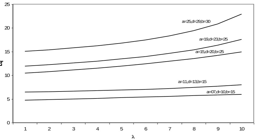
The expected number of customers in the queue can be computed for varying with fixed a, d, b, and . The nature of the curve is exhibited in the following graphs. For this model one can draw countless number of curves by changing the unknown parameters a,d,b, and We have exhibited the curves by taking the values of (a,d,b) as (07,10,15),(11,13,15), (15,20,25), (19,23,15) , (25,29,30) and =0.5 for the following three cases:
(i)
(ii)
(iii)
The mean queue length (Lq) for different values of are shown in the following table 1 and their corresponding curves are exhibited in figures 1,2 and 3.
a=7,d=10, b=15 a=11,d=13, b=15 a=15,d=20,b=25 a=19,d=23,b=25 a=25,d=29,b=30
8 10 10 8 10 10 8 10 10 8 10 10 8 10 10
10 10 8 10 10 8 10 10 8 10 10 8 10 10 8
1 4.75 4.74 4.76 6.44 6.44 6.47 10.44 10.42 10.48 11.95 11.93 11.99 15.05 15.03 15.09
2 4.88 4.87 4.92 6.52 6.53 6.59 10.78 10.75 10.89 12.26 12.24 12.38 15.40 15.37 15.52
3 5.00 4.99 5.08 6.62 6.63 6.73 11.15 11.11 11.36 12.62 12.58 12.84 15.80 15.76 16.06
4 5.13 5.12 5.26 6.72 6.74 6.91 11.54 11.50 11.91 13.01 12.98 13.41 16.27 16.22 16.74
5 5.25 5.26 5.45 6.84 6.87 7.13 11.96 11.93 12.54 13.46 13.43 14.13 16.83 16.78 17.63
6 5.38 5.40 5.65 6.97 7.03 7.41 12.41 12.41 13.29 13.97 13.97 15.06 17.49 17.46 18.87
7 5.50 5.54 5.87 7.12 7.21 7.80 12.89 12.93 14.18 14.56 14.61 16.31 18.28 18.31 20.70
8 5.63 5.68 6.11 7.28 7.42 8.33 13.41 13.52 15.27 15.25 15.39 18.10 19.28 19.40 23.64
9 5.75 5.83 6.37 7.48 7.68 9.14 13.96 14.17 16.63 16.07 16.34 20.85 20.53 20.85 29.20
[image:4.595.58.542.423.702.2]0 5 10 15 20 25
1 2 3 4 5 6 7 8 9 10
Lq
a=25,d=29,b=30
a=19,d=23,b=25
a=07,d=10,b=15 a=11,d=13,b=15
[image:5.595.69.509.79.340.2]a=15, d= 20,b=25
Fig. 1. Mean queue length Vs for different values of a, d and b when
0 5 10 15 20 25
1 2 3 4 5 6 7 8 9 10
Lq
a=25,d=29,b=30
a=19,d=23,b=25
a=07,d=10,b=15 a=11,d=13,b=15
a=15,d=20,b=25
[image:5.595.71.513.381.622.2]0 5 10 15 20 25 30 35 40 45 50
1 2 3 4 5 6 7 8 9 10
Lq a=25,d=29,b=30
a=19,d=23,b=25
a=07,d=10,b=15 a=11,d=13,b=15
[image:6.595.67.519.111.370.2]a=15,d=20,b=25
Fig. 3. Mean queue length Vs for different values of a, d and b when
The above figures reveal that the Lq increases when increases. Similarly when fixing , for varying (a, d, b), the values of Lq increase. In addition to that, Lq varies according to the nature of Now considering the three cases:
Lq is lower when higher when and lies between the above two cases when
4. REFERENCES
[1] CHAUDHRY, M.L and TEMPLETON, J.G.C (1983), A first course in Bulk service queues, John Wiley. New York.
[2] GANESAN, V. (1999), Steady state solutions for Erlangian queques with general bulk service rule, Journal of Kerala Statistical Association, Vol : 10, 22 - 28 [3] GOHAIN. S, and BORTHAKUR, A. (1979), On
difference equation technique to bulk service queues with the server, Pure Appl. Math. Sci. X(1-2), 40 –46
[4] GROSS. D. and HARRIS . C.M. (1985), Fundamentals of queueing theory, John Wiley, New York.
[5] KAMBO, N.S. and CHAUDHRY, M.L. (1985), Single server bulk services queue with varying capacity and Erlang Input. INFOR, 23,196-204.
[6] MEDHI. J. (1984), Recent developments in Bulk Queueing Models, John Wiley Eastern Limited.
[7] NEUTS, M.F. (1967), A general class of Bulk queues with Poisson input, Annals. of Math. Statistics, 38, 759-770.