Public Good Provision: Using an Evolutionary Game Theoretic Approach to Modeling

(1)

Munich Personal RePEc Archive

Public good provision : using an

evolutionary game theoretic approach to

modeling

Sandeshika, Sharma

University of California, Irvine

2004

(2)

Public Good Provision: Using a Qualitative

Evolutionary Game Theoretic Approach to

Modeling

Sandeshika Sharma

August 11, 2004

Abstract

In studying interactions among multiple agents or strategies, the equilibrium predictions almost always depend on the the specific mod-elling details. Though choosing specific functional forms can aid intu-ition and give useful insights about the underlying social or economic phenomenon, realistically arguing, we can rarely capture the richness of the social or economic interactions with any specific functional form.

To overcome the problem of functional form dependence of equilib-rium predictions, we employ a newly developedQualitative Evolution-ary Game Theoretic Approach (Saari, 2002) to give us results that are robust to any choice of functional specification. The QEGT approach can potentially give us all possible models of agent interactions, if we specify the near-equilibrium behavior.

In this paper I examine models of public good provision and show how the QEGT approach allows us to go beyond the existing game theoretic and quantitative evolutionary game theoretic approaches, in terms of predicting all the existing and many new plausible equilibria.

(3)

1 Introduction

In the area of game theoretic modeling, we often encounter the issue of multiple agents or multiple strategy interactions. Modeling becomes even more compli-cated if the underlying game is dynamic in nature. A common problem we face while studying interactions among multiple agents or strategies is that equilibrium predictions almost always depend on the the specific modelling details. As an ex-ample, in a model of public good provision, the different equilibria the models predict are contingent on choice of functional forms.

Though choosing specific functional forms can aid intuition and give useful in-sights about the underlying social or economic phenomenon, realistically arguing, we cannot capture the richness of the social or economic interactions with any specific functional form. The only time we can “reliably” use a specific functional form is when we have fairly precise information about the variables and inter-actions leading to a particular phenomenon. Such precise information is rarely available in the social sciences.

To overcome the problem of functional form dependence of equilibrium pre-dictions, we employ a newly developed Qualitative Evolutionary Game Theoretic Approach(Saari, 2002) to give us results that are robust to any choice of functional specification. By using the Qualitative Evolutionary Game Theoretic Approach, we can learn about the generic equilibria of the system, rather than only the spe-cific equilibria (which are predicted by models described by spespe-cific functional forms).

We basically adopt a new approach to specifying models. We specify models based on the concept of “local information”. (In traditional modeling, models are specified using specific functional forms.) Local information corresponds to infor-mation about the direction of dynamics, near the plausible equilibria of the model. Local information also serves the function of assumptions in traditional modeling. After specifying the local information, we either apply the Intermediate Value the-orem or compute the Winding Number of the dynamical system (depending on the strategy dimensions) to determine the equilibria of the model.

(4)

can qualitatively characterize the paths leading to different equilibria. This makes QEGT a useful tool for policy; the QEGT approach allows us to study global consequences of local policy changes.

The alternative to the QEGT approach is to explicitly find (or simulate) the solution to a complicated system of differential or difference equations, where the equations are based on a specific functional form. Moreover, a useful property of the QEGT approach is that the results are not sensitive to changes in functional forms; as long as we can gather local information accurately, it is sufficient to give us insight about the global behavior of the system.

In this paper we use the QEGT approach, to understand the dynamics of a widely studied game—the game of voluntary provision of public goods. The variant of the public good game we study involves interaction among three types of agents—cooperators, loners and free-riders. While most analyses of public good games focus attention on only two types of agents or strategies1

, we focus attention on interactions among these three strategies. We want to address questions of the following type: 1. How do different agents in the population interact? 2. What type of equilibria do the different interactions produce? 3. Under what situations, cooperation is likely to evolve? 4. Can we design policies to raise the likelihood of cooperation?

1.1 Paper Outline

In section 2 we begin the analysis by making a case for employing evolutionary game theoretic approach over traditional game theoretic approach. Here we also outline the basic difference between game theoretic and evolutionary game theo-retic approach. We also briefly introduce the Qualitative Evolutionary Game The-oretic Approach, and discuss how it differs from quantitative evolutionary game theoretic approaches. In section 3 we begin by explaining the basic modeling framework. We show how the QEGT approach works. We characterize the differ-ent equilibria that emerge from interaction of the three strategies—cooperators, loners and free-riders. In section 4 we study policies designed to raise likelihood of cooperation in public good provision. Here we also discuss how in absence of global dynamics, policy makers can make inaccurate recommendations. Section 5 concludes. All figures are in the appendix.

1

(5)

2 Methodological Background

2.1 Evolutionary Game Theoretic Approach

Evolutionary game theoretic explanations are being increasingly used to study social and biological systems. While the evolutionary game theoretic approach comes from biology, it is emerging as an important modelling paradigm within the social sciences. A wide range of individual behaviors and phenomenon which hith-erto could not be accounted for, following the predictions of standard game theory can be explained elegantly using the evolutionary game theoretic approaches. For instance, evolutionary game theoretic approaches are shedding new insights on is-sues concerning emergence of justice (evolution of the equal sharing norm, (Skyrms (1994)), evolution of social conventions and norms for reciprocity (Young (2001)), evolution of cooperation in prisoner’s dilemma game and more recently evolution of cooperation in public goods provision (Hauert (2002) et.al). Let us look at some of the differences between the Game Theoretic and Evolutionary Game Theoretic paradigm.

2.2 Game Theory versus Evolutionary Game Theory

2.2.1 Notion of Equilibrium and Multiple Agents

The notion of equilibrium in game theoretic framework differs fundamentally from the notion of equilibrium used in evolutionary game theory. Within the game theoretic framework, individual strategies are assumed to be optimal given ex-pectations, and expectations are assumed to be justified given the evidence. In evolutionary game theoretic approaches however, equilibrium is understood within a dynamic framework that explains how the equilibrium comes about (Rephrased from Young, (2001)).

(6)

2.2.2 Rationality

As mentioned earlier, game theory assumes that players are fully rational and choose the strategy that gives the highest expected utility over time, given their expectations about what the other players will do. Unlike the standard game theo-retic approaches, the evolutionary game theotheo-retic approach is based on a different model of human behavior. The essential idea of the evolutionary game theoretic approach can be summarized with the following comment from Young (2001):

Agents adapt—they are not devoid of rationality—but they are not hyper-rational. They look around themselves, they gather informa-tion, and they act fairly sensibly on the basis of their information most of the time. In short, they are recognizably human. Even in such “low-rationality” environments, one can say a good deal about the institutions (equilibria) that emerge over time. In fact, these in-stitutions are often precisely those that are predicted by perfect equilib-rium, Pareto-efficient coordination equilibria, the iterated elimination of strictly dominated strategies and so forth. In brief, evolutionary forces often substitute for high (and implausible) degrees of individual rationality when the adaptive process has enough time to unfold.

The evolutionary game theoretic approach therefore relies on a primitive model of agent behavior; agents are in a learning environment. Strategies that emerge successful in evolutionary competition (much like the biological evolution model) become established.

2.2.3 Dynamics

(7)

consider a wider range of learning rules (or dynamics)—best response, imitation, replicator dynamics.

Result of evolutionary game theoretic modelling however are often sensitive to the assumption about the dynamic learning rules. Moreover analytical predictions are often difficult to get, since the models typically involve complicated differential or difference equations. A common way to avoid explicitly solving the differen-tial equations is to run simulations. The equilibrium predictions are often made based on simulation results. In this context, it is useful to look at a qualitative approach to evolutionary game theory. This qualitative approach overcomes some of the mathematical intractability of quantitative evolutionary game theoretic ap-proaches.

2.3 Qualitative Evolutionary Game Theoretic Approach

The Qualitative Evolutionary Game Theoretic approach (Saari (2002)), enables us to get analytic predictions for the all different equilibria of a game, without having to explicitly solve complicated differential equations or rely on simulations. This way, the qualitative approach can strengthen the predictions from existing quantitative and simulation based approaches within evolutionary game theory. In the following section, we illustrate how the QEGT approach works using the example of public good provision. In practice, the QEGT approach involves gen-erating the “local information”2

and calculating something known as the Winding Number (a higher dimensional counterpart of the Intermediate Value Theorem) for a given dynamical system. To generate local information, we essentially need to make assumptions about the direction of local dynamics in the neighborhood of a particular equilibrium. The winding number gives us information about the global dynamics of the underlying dynamical system.

It is crucial to note that in absence of the QEGT approach,the researchers would need to explicitly solve complicated differential equations to learn about the equilibrium behavior of the dynamical system.

A useful aspect of the QEGT (over the game theoretic and quantitative evo-lutionary game theoretic approach) is that the predictions made using the QEGT remain unchanged if there are different analytical representations of the same un-derlying phenomenon. This is crucial since in social sciences where we often lack directly verifiable primary data sources. If the model predictions depend on a par-ticular functional specification (say quadratic or cubic), then our inference about

2

(8)

the phenomenon would be limited by the mathematical properties of the functional form we use.

Now we will apply the QEGT approach to study the voluntary provision of public goods problem.

3 Framework

In this section we will study the social dilemma involved in public good provision. We will use the following illustration to outline the public goods game: consider the construction of a public park through voluntary contributions. A community is debating whether they want to convert a piece of unused land into a public park. We can guess that the public park will not be built unless a certain fraction of the agents support the project. Our framework consists of three different kinds of economic agents—cooperators, free-riders and loners.3

.

Cooperators are agents who fully support the public park project. They are willing to make contributions towards converting the unused land into a public park. Free-riders on the other hand, can be thought of as users of the park who declare themselves to be cooperators but, in fact, do not contribute. According to our framework, while the cooperators support the public park “loners” refrain from participation. The loners are to be viewed as skeptics, who can be persuaded to join, but on their own consider the odds of success for the public park project to be slim. The reason loners are skeptical can be attributed to at least two factors. Firstly, loners worry that most people will choose to be free-riders. Secondly, even if there is relatively low free-riding, the loners are unsure if there are enough agents willing to make the initial investment.

We ask the question whether there is a way to determine all possible models of interaction between Cooperators, Loners and Free-riders. The QEGT approach allows us to determine all possible models of interaction between cooperators, lon-ers and free-ridlon-ers as long as the strategy adjustment dynamics is assumed to be continuous.

To execute the QEGT approach we need “local information” near the plausible equilibrium. Let us now define what we mean by local information.

3

(9)

Definition 1 (Local Information) Local Information corresponds to the direc-tion of dynamics, near a plausible equilibrium of the system.

For this purpose, we begin by studying the pairwise interaction dynamics among the three strategies: cooperator, loner and free-rider.

3.1 Generating Local Information

3.1.1 Pairwise Interaction: Cooperators and Loners

Consider a population that consists only of cooperators and loners. For simplicity, let us study the game by considering the pairwise interaction among the three strategies. First let us look at the interaction between cooperators and loners. The two strategies can be represented by pointsLandC along the segmentL−C

in figure 1.

Figure 1 about here.

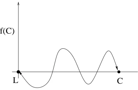
Figure 1 tells us that if we are at pointL, the entire economy consists of lon-ers; at pointCon the other hand, the entire economy consists only of cooperators. If we are close to point L then the economy consists mainly of loners and a few free-riders. Now we go to the next step.

In one possible scenario, if there are too many cooperators in the economy it may happen that the loners will be motivated to become cooperators since they are confident that the public good project would succeed. On the other hand, if there are too many loners or skeptics, even the willing cooperators may get discouraged and become skeptical, after seeing the low levels of participation. In other words, if there are too many loners, and very few cooperators, the loner strategy may come to dominate and cooperative behavior would eventually disappear. This informa-tion is represented in figure 2. Figure 2 tells us that the model of interacinforma-tion of loners and cooperators has at least two plausible equilibria: one with all loners and second with all cooperators. The behavior of the dynamic near the equilibria, all cooperator and all loners is represented by figure 2. The arrows near the equilibria indicate the direction of movement of the dynamics. The dynamics is measured along the vertical axis by the function f(C).

(10)

ap-proach gives us a way to determine all other equilibria of this system.

Using the Intermediate Value Theorem

If we assume the dynamics to be continuous, figure 2 shows us how to interpret the equilibrium points L and C. At the equilibria pointsL and C, the dynamics (as represented by f(C) in figure 2) has a value zero. If the horizontal axis in figure 2 measures the proportion of cooperators in the population and the vertical axis (or f(C)) measures the rate of change of population of the cooperators, we can infer the following: near equilibriaL, the dynamics (or rate of change of pop-ulation of cooperators) must be negative, since atL, the population proportion of cooperators drops to zero. Similarly near equilibria C, the dynamics must have a positive value, before it attains a value of zero, at the equilibrium point C. This information is represented by the arrows in figure 3.

Figure 3 tells us that if the function f(C) (measured along the vertical axis) is continuous, then by the Intermediate Value Theorem, it must be the case that the population rate of change dynamicsf(C) intersects the horizontal axis at least once. In fact, in general, the dynamics can intersect the horizontal axis more than once; generically speaking, the dynamics can intersect the horizontal axis an odd number of times. Figures 4 and 5 show one and three intersections of f(C) with the horizontal axis respectively.

Figure 4 and 5 about here.

For simplicity let us assume that the dynamics intersects the horizontal axis only once. With that scenario, we can now fully characterize all the equilibria of the model studying interactions among loners and cooperators. In particular, the loner-cooperator interaction model will have another equilibria, denoted by point P, and it will be unstable in nature. This is represented by figure 7.

3.1.2 Pairwise Interaction: Cooperators and Free-riders

(11)

of the public good would very small. The free-riders would exploit the cooperators and this causes the cooperators to stop investing in the public good.

Now let us consider the interaction dynamics between cooperators and free-riders. Foreseeing the difficulty of cooperation emerging as a stable equilibrium in presence of free-riding, assume that the cooperators design a system of monitoring. Let us suppose the system works in the following way: With some probability, a free-rider will be apprehended by a patrol officer hired by the cooperators.

The importance of the monitoring device is to ensure that for some value of the patrolling probability, the expected return of a free-rider will fall below the expected return of a cooperator. Therefore, in the setting where there is a large percentage of cooperators, the expected return to free-riding fall below the returns to cooperation; at this stage, free-riders would have an incentive to choose co-operation. As a result, cooperation emerges as a stable equilibrium. The above situation is represented in figure 8.

Figure 8, about here.

On the other hand, it is reasonable to assume (as indicated in Figure 8), that if the society is dominated by too many free-riders, patrolling is ineffective. So, while with relatively fewer free-riders, free-riding can be contained, a society dominated by free-riders, will crush cooperation.

The interesting fact is that following these assumptions, the Intermediate value theorem mandates the existence of another equilibrium, given by pointM. Again according to the QEGT approach the generic properties of this equilibrium suggest that it should be unstable. This means M serves as a threshold point where on one side of M, society tends to the free-riding state, on the other side it tends towards universal cooperation.

3.1.3 Pairwise Interaction: Free-Riders and Loners

In the final pairwise analysis, we need to characterize the interaction in a society consisting strictly of loners and free-riders. This society has no public goods, so nothing happens. On the other hand, with a small amount of public good, (with cooperators in the minority and no monitoring) free-riders will prevail. This pair-wise interaction is represented by figure 9.

(12)

3.1.4 Overall Interaction: Cooperators, Free-Riders and Loners

The next step is to fully characterize the interactions between the three strategies: cooperator, loner and free-rider. What other equilibria do we get? To answer this question, we will calculate the winding number for the given dynamical system. In any typical dynamical model, we would need to solve a set of complicated dif-ferential equations to determine the interaction dynamics. The QEGT approach however works on information from local dynamics.

Based on the model, in figure 7 and 8, we extracted information about the local dynamics around the loner, cooperator and free-rider equilibria. The local information tells us that the L, C and F equilibria are stable in the pairwise in-teraction. Additionally we have two more equilibria along the L−C and C−F

edges— P and M- both of which are unstable. Let us represent this situation using the simplex in figure 10.

The simplex represents all the different equilibria. For instance,L represents the equilibrium with all loners. Similarly,P represents the equilibria with a certain fraction of population consisting of cooperators and the remaining consisting of loners. Note that there is no interaction dynamic along the loner-free-rider edge. But what about the dynamics close to the L−F edge? Close to the L−F edge,

there are very few cooperators and a majority of loners and free-riders. We assume that close to the L−F edge, the free-riders prosper, relative to the loners and

cooperators.4

We now show that from the pairwise interaction dynamics, we can identify the interaction dynamics among the three strategies. To begin consider a situation with is a very small percentage of free-riders in a population; the population con-sists mainly of loners and cooperators. Then there are different possibilities for the free-riding strategy. Either free-riders would prosper or disappear over time. From the above model, in this way we can characterize what happens close to the edges L-C, F-C and L-F.5

In specific, four possible scenarios can be outlined,

4

Note that with a change in this assumption about the dynamics, we will get the corresponding results.

5

Note that we have already assumed the overall behavior of the dynamics near theL-F

(13)

which correspond to four different public good games. We list them below:6

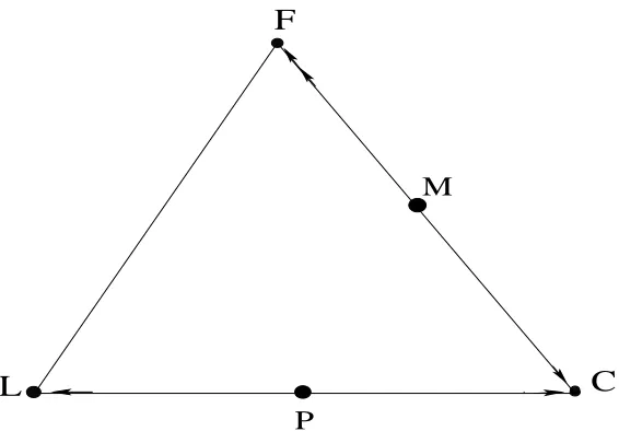
1. When the system is near equilibria P, free-riders tend to prosper. A sup-porting argument is that the population consists primarily of loners and cooperators, so with lack of attention placed on free-riders, they have an opportunity to exploit the system. In this situation, free-riders prosper over time. This is represented by the dynamic pointing away fromP. See figure 11.

Next we need to consider what happens nearM. NearM, the society essen-tially consists of free-riders and cooperators. Since the public good project is supported, it is reasonable to assume that the hitherto skeptical loners will commit- either to cooperate or to free-ride. Therefore, the dynamic is pointing towards M, along the F-C edge.

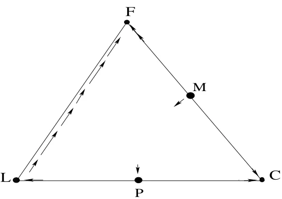
2. A second scenario starts with the same assumption about the system be-havior near equilibrium P, thus the free-riders tend to prosper. Therefore, the dynamic is pointing outwards from point P. On the other hand, when the system is near the equilibria denoted by M, loners tend to prosper; this could occur if the co-existence of free-riders and cooperators generates doubts about the success of the public project. This encourages more people to become loners. So when the system is near M, loners tend to grow in percentage terms. This is indicated by the dynamic pointing away fromM. See figure 12.

3. Consider a situation where the population consists mainly of loners and co-operators; let the environment be such that when there are relatively few free-riders, moral or social pressures force them to give up free-riding. This situation is illustrated by the dynamic in figure 13, pointing towards P. In other words, the system is such that when the system is near equilibria P, free-riders tend to disappear. Let us assume the same behavior for the in-teraction dynamic when the system is nearM; i.e. the loners disappear over

towardsF; i.e. the free-riders tend to prosper over time.

6

(14)

time. As a result the dynamic is pointing towardsM.

4. In the last scenario, we assume a situation such when the system is near equilibriaP, free-riders tend to disappear, as assumed in scenario 3. There-fore, the dynamic is pointing towardsP. As for the behavior of the dynamics near M, we assume that over time loners tend to prosper. This is the same assumption that we made in scenario 2. This is illustrated by the dynamics pointing away fromM in figure 14.

The four scenarios are four different public good games and allow us to capture a wide range of dynamic interactions. In the subsequent section, we study how to generate information about the global dynamics of these public good games, based on the local information we extracted above.

3.2 Analysis of Global Dynamics

The important fact is that scenarios 1 through 4 fully characterize the above model. With this information about the local dynamic, can we make any statements about other equilibria of the system? The next step is to calculate the winding number for each of the four scenarios to determine if there are any more equilibria of the system. Following the method described in the Appendix I, we can compute the winding number for scenario 1. The winding number equals +1. The winding number equals the sum of indices of local equilibria. From the Index theorem it follows that there may not be any more equilibria of the system. The global dynamics is illustrated in figure 15.

(15)

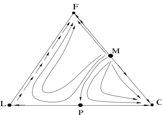
Consider scenario 2. The winding number equals +2. Sum of the indices of the local equilibria equals +3. The Index theorem tells us that there must be at least one saddle equilibrium inside the simplex; this is due to the fact that sum of local indices of the equilibrium must equal the winding number of the dynamical system. Scenario 1 is represented by figure 16.

Figure 16 expresses the following situation- If there are very few loners and free-riders in the population, the system evolves to full cooperation. There is a finite chance that the system will evolve to the saddle equilibrium. If there are more than a certain fraction of loners or free-riders however, the system will always evolve to a situation of full-free-riding.

Figures 17 and 18 show all the other equilibria and the global dynamics corre-sponding to the scenarios 3 and 4. If the system is within the basin of attraction of full cooperation, it will evolve to full cooperation, else it will evolve to free-riding.

4 Policy Intervention

Let us now assume that there is an upper bound on the extent of monitoring that the cooperators can provide. If this is the case, then public policy can play a constructive role in raising the level of cooperation, by either increasing the mon-itoring of the public good or by giving incentives to the loners to participate in public good production. In this section, we consider two policies to enhance the level of cooperation; first raising the extent of monitoring activity and second, giving incentives to loners to become cooperators.7

Note that we will study policy in a qualitative way. It is important to recognize the role of policy here; policy is seen as an instrument that complements the efforts of cooperators. It is meant to support and increase the likelihood of successful provision of public good, and not provide public goods.

The QEGT approach allows us to study policy through a new approach. Pol-icy recommendations are made after examining the interaction dynamics among the different strategies. We claim that traditional policy analysis will not be able to distinguish between alternative policies unless it simultaneously studies the

dy-7

(16)

namic path of policy. We show that in many situations policy intervention is not required, but a well meaning policy maker may nonetheless expend resources in intervention. In such a situation, it is clearly not enough to study the different equilibria of the system: we need information about the dynamic paths leading to different equilibria.

Note that the global analysis of policy implications is made possible by the QEGT approach. In absence of this tool, undertaking a systematic dynamic anal-ysis of policy is seldom feasible. In the present context, policy is seen as an instrument to bring about new equilibria within the system. Alternatively, it can be seen as an instrument that reduces the likelihood of an unfavorable state.

Here we are looking for policy intervention that raises the likelihood of coop-eration and/or enables an economy evolving to an unfavorable equilibria to reach the socially desirable state. We assume that achieving highest possible level of cooperation is a desirable social objective.8

4.1 How Policy Works

We assume that the policy maker has information about the population proportion of the three strategies- cooperation, loner and free-riding. Here we consider a few instruments policy makers can use to raise cooperation.

We first show that by changing the monitoring probability, and by giving in-centives to loners to become cooperators, the basin of attraction of cooperation can be modified. Let us see how these two policies work.

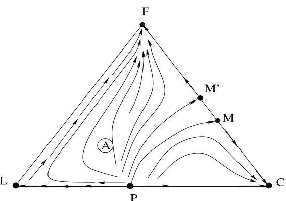
First, consider the policy of raising the monitoring probability. In figure 19, the location of the interior equilibrium point on the free-rider–cooperator edge is left undetermined within our qualitative framework. However, as monitoring probability goes up, it increases the basin of attraction of the cooperation strat-egy, along the C₋F line. The new basin of attraction of cooperation is given by the region M′_C.

Second, consider the policy of giving incentives to loners. In this situation, let us look at the loner–cooperator edge in figure 20. By giving incentives to loners to become cooperators, the basin of attraction of cooperation increases and the

8

(17)

interior equilibrium along the L-C edge shifts to the left.

After understanding the basic consequences of policy, let us consider a few sce-narios under which public policy can be implemented to raise the level of public good production. We also discuss situations where public policy will be counter-productive.

In policy analysis we also study the implications of increase in centralization in government decision making on voluntary provision of public goods. At a qualita-tive level, increase in centralization can lower the productivity of the public goods. This would lower the basin of attraction of cooperation strategy along the L₋C edge. While centralization of decisions is an important instrument for coordinating decisions in any economy, a high degree of centralization can undermine citizen preferences, and cause unnecessary delays in project implementation. In extreme situations, it can also crowd out voluntary cooperation altogether.

In the following section, we discuss how policy should be designed. We show the consequences of designing policy without paying attention to the global dynamics of the system. For illustration, the analysis is done only for scenario 1. It easily generalizes to scenarios 2 through 4.

4.2 Policy Analysis

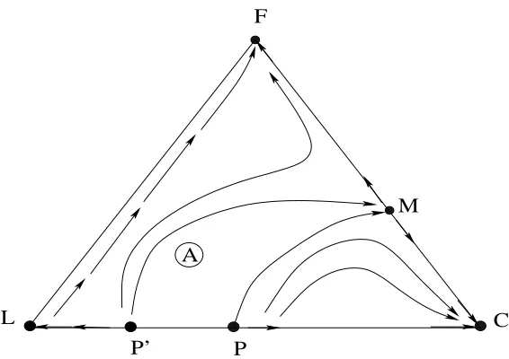
Case I Consider point A within the simplex, in Figure 21; it indicates the cur-rent state of an economy or social system. Since point A lies outside the current basin of cooperation strategy (as determined by the maximum level of monitor-ing cooperators can afford), if the policy maker doesn’t intervene, the system will eventually evolve to the degenerate equilibrium of failure of cooperation.

Figure 21 and 22, about here.

The question however is, what policy instrument is to be used in this situation. We claim that the most appropriate instrument here involves giving incentives to loners. Relying on raising the extent of monitoring will not have any impact on raising the level of cooperation. Figure 22 shows that if we give incentives to lon-ers, it changes the basin of attraction of the cooperation strategy. The interior equilibrium shifts from pointP toP′_{. Note that point}_{A, now lies within the new}

(18)

until full cooperation evolves.

Figure 23, shows what happens if the policy maker responds to the present state of the economy by raising the monitoring probability. On the F-C edge, the new interior equilibrium would be to atM′_{, instead of being at} _{M. But note that}

if the internal dynamic has the behavior as indicated by figure 21, the economy will still evolve to the degenerate equilibria, since the path of the policy has not affected the path of evolution of the economy. In this case, policy intervention is completely ineffective in raising the level of public good provision. If the policy maker responds by giving incentives to loners, the policy will have no impact on raising the level of public good provision. In fact, over time, the system will evolve to the degenerate equilibrium.

What we observe here is that traditional approach to policy making will not be enable the policy maker to select the appropriate policy, unless they have any information about the dynamic paths. The point is that we can undertake more informed policy making if we have information about the global impact of any specific policy.

Case II Consider pointB in figure 24. If policy maker responds by raising the extent of monitoring, it increases the basin of attraction of cooperation such that the new equilibria along the edge shifts from M to M′_{. Note that the new basin}

of attraction (figure 25) of cooperation includes point B. Therefore, even though there will be an increase in proportion of free-riders in the population, as the economy evolves from point B, it will be only be temporary and with time. The economy will be able to reach the full cooperation.

Figures 24, 25 and 26 about here.

If on the other hand, the policy maker responds by giving incentives to loners, policy will have no impact on raising the level of public good provision. This is because, the new basin of attraction of C does not include point B. In fact, over time, the system will evolve to the degenerate equilibrium. Figure 26, shows the situation where policy is misplaced and ineffective.

(19)

pop-ulation. Then the level of loners peaks at some point and begins to go down. Thereafter, the proportion of free-riders peaks at some point, after which it begins to go down on its own, until both free-riders and loners go extinct and the full cooperation is achieved.

If policy maker is unaware of the highly non-linear dynamic inside the simplex, and he recommends giving incentives to loners to take the economy from pointD to C, then such a policy is unnecessary. If the path of policy is as indicated in figure 27, then regardless of the policy, the economy will evolve to the full cooper-ation equilibrium.

Case IVLet pointE, in figure 28 represent the current state of the economy. Note that point E lies within the basin of attraction of cooperation. In this situation, there is clearly there is no need for policy intervention. The policy maker however, observes that the proportion of free-riders is growing over time. Since he does not see the overall dynamics within the simplex, the policy maker may intervene with the intention of raising the likelihood of cooperation. If he responds by increasing the level of government involvement in the project, in terms of asking for project updates and plan layouts, it may create bureaucratic delays and create opportu-nities for bureaucratic corruption.

Figure 28 and 29, about here.

Therefore, in this situation, raising the level of government involvement can adversely affect the returns from the public good. Increasing the level of gov-ernment involvement or greater centralization can cause the some local changes around point E such that it is now more costly to adopt cooperation. In such a situation, it might be the case that point E, now lies outside the new basin of cooperation, since the boundary of the basin shifted due to the local change in government policy. In this situation, public policy would crowd out voluntary initiative and cooperation.

(20)

a road, the repair of a school building, and construction of a community center. Hinderance arose when such projects had to be put on hold, until permission was granted from the state government authorities.

Notice how in these settings, the public good problem does not occur from free-riding. Instead, the problem is caused by over-centralization of the public decision making structure. This suggests that beyond a resource constraint in the full provision of public good by governments, a more pertinent factor is the cost of fully centralized decisions. Such decisions often undermine citizen preferences and may even thwart voluntary citizen initiatives. This fact is being increasingly recognized in recent literature (Pinkerton (1989), Watson (1995), Wunsch and Olowu (1995), Ostrom (1997)).

5 Results and Discussion

In the above analysis we see how the QEGT approach (potentially) allows us to get all possible models of interaction between cooperators, loners and free-riders. In section 3, based on the specification of the local information, we describe four models of cooperator, loners and free-rider interactions. After outlining the global dynamics of the models, we address the issue of raising the likelihood of reach-ing the cooperative equilibrium through policy intervention. Since our dynamic approach allows us to characterize the interaction among different strategies, this gives us a useful tool while designing policies. After having this information, we can study the global implications of any policy. In absence of the information about the global dynamics, we show that policy makers can often make incorrect recommendations about the most suitable policy. In section 4.2 we saw how policy maker can respond by selecting the wrong policy, in absence of having information about the dynamics inside the simplex.

The information about the path of a policy, or the global dynamics is made available to us by QEGT approach. If the path of a policy is well understood, it can save resources and time spent in solving problems. Therefore by studying the path, we get an insight into the appropriate design of policy.

(21)

the quantitative and qualitative approaches can work synergistically to improve our understanding of social and economic phenomenon. It is important however, to recognize that the reliance on only a quantitative approach will give us results that are based on functional specification of the model. In order to get a fully general understanding of the different equilibria of a model, we should use the QEGT approach.

References

[1] Axelrod, Robert.The Evolution of Cooperation,Basic Books Inc. Publishers, New York, 1984.

[2] Ellison, G. Learning, local interaction and coordination, Econometrica,61

(1993), 1047-1072.

[3] Hauert, Ch., De Monte, S., Hofbauer, J. and K. Sigmund. Volunteering as Red Queen Mechanism for Cooperation in Public Good Games Science,296

(2002), 1129-1132.

[4] Ostrom, Elinor. Crossing the Great Divide: Coproduction, Synergy and De-velopment, in Peter Evans eds State-Society Synergy: Government and Social Capital in Development, University of California Press/University of California International and Area Studies Digital Collection94 (1997), 85-118.

[5] Pinkerton, Evelyn. Cooperative Management of Local Fisheries: New Direc-tions for Improved Management and Community Development, Vancouver, University of British Columbia Press, 1989.

[6] Saari, Donald G. Mathematical Social Sciences An Oxymoron?, Lectures at Pacific Institute of Mathematical Science, 2002.

[7] Sharma, Sandeshika. Essays in Political Economy: Using a Qualitative Evo-lutionary Game Theoretic Approach. Phd Dissertation, University of Cali-fornia, Irvine, 2004.

[8] Skyrms, Brian. Evolution of Social Contract, Cambridge University Press, 1996.

(22)

[10] Watson, Gabrielle. Good Sewers Cheap? Agency-Customer Interactions in Low-Cost Urban Sanitation in Brazil, Washington D.C.: World Bank, Water and Sanitation Division,1995.

[11] Whitaker, Gordon P. Coproduction: Citizen Participation in Service Deliv-ery, Public Administration Review,40 (1980), 240-46.

[image:24.612.192.418.129.276.2]

f(C)

Figure 5: Global Dynamics-Three Interior Equilibria-L and C

C

L

f(C)

[image:24.612.192.421.378.529.2]

(25)

P

L

[image:28.612.163.447.371.572.2]

(29)

P

M

F

C

L

[image:29.612.165.447.89.287.2]

R

Figure 15: Global Dynamics for Scenario 1

P

M

F

C

L

[image:29.612.164.446.371.571.2]

(30)

P

M

F

[image:30.612.165.447.89.286.2]

C

L

Figure 17: Global Dynamics for Scenario 3

P

M

F

C

L

[image:30.612.163.444.371.570.2]

(31)

L C P

F

[image:31.612.160.447.89.286.2]

M M’

Figure 19: Policy Intervention-Raising Monitoring Probability

M

F

C

L

P’

P

[image:31.612.162.447.371.573.2]

(32)

L C P

F

M

[image:32.612.164.446.89.288.2]

A

Figure 21: Economy at A, evolves to F

L C

P F

M

A

P’

[image:32.612.163.446.372.572.2]

(33)

L C P

F

M

A

[image:33.612.164.447.87.286.2]

M’

Figure 23: Policy Intervention Ineffective

L C

P F

M B

[image:33.612.164.449.369.571.2]

(34)

L C P

F

M M’

[image:34.612.164.446.89.289.2]

B

Figure 25: Policy Intervention-Economy evolves to C

L C

P F

M

P’

B

[image:34.612.163.445.371.573.2]

(35)

P

M

F

C

L

[image:35.612.164.447.89.287.2]

D

Figure 27: Highly Non-linear Dynamics

L C

P F

M

E

[image:35.612.163.446.372.571.2]

(36)

L C P

F

M

E

[image:36.612.163.448.232.429.2]

P’