Optimization of Wireless Sensor Network Lifetime by
Deploying Relay Sensors
B.Brahma Reddy
ECE, VBIT, Aushapur, Ghatkesar, RngaReddy district Hyderabad, India-501301
K.Kishan Rao
Director, Vaagdevi College of Engineering Bollikunta, Warangal, India- 506005
ABSTRACT
Topology control in wireless sensor networks helps to lower node energy consumption by reducing transmission power and by confining interference, collisions and consequently retransmissions. Decrease in node energy consumption implies probability of increasing network lifetime. In this paper, firs popular topology control algorithms are used for analyzing optimizing the power consumption in the wireless sensor network and later proposed a novel technique wherein power consumption is traded with additional relay nodes. Later relay nodes are introduced to make the network connected without increasing the transmit power. The relay node decreases the transmit power required while it may increase end-to-end delay. This paper designs and analyzes an algorithm that place an almost minimum number of relay nodes required to make network connected. Greedy version of this algorithm is implemented and demonstrated in simulation that it produces a high quality link. InterAvg, InterMax (no of nodes that can offer interference) MinMax, and MinTotal are used as metrics to analyze and compare various algorithms. Matlab and NS-2 are used for simulation purpose.
Key Words
Energy saving, sensor networks, Interference, network connectivity, topology control
1.
INTRODUCTION
Sensor network applications became popular due to their easy and rapid deployment processes. They can be deployed even into hazardous environments. These networks monitor outdoor environments and provide crucial data for emergency situations. Hence network connectivity is utmost important. They also work under extreme conditions such as noise and hostile atmosphere. They must work with minimum energy so that they work longer periods and offer minimal interference. Topology control can play major role in reducing node power consumption and extend network life time. In order to conserve the energy, the nodes are preferably configured at low transmit power. When the sensors are deployed at random locations, each node is to be configured at different transmit power levels making the network heterogeneous. However, it is possible to make the network homogenous by adding additional relays nodes at certain places which also conserve the network energy.
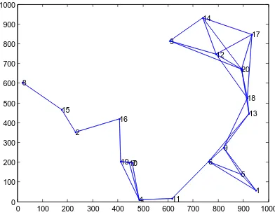
An efficient and energy conservation multi-hop wireless sensor network is discussed here. If the node are deployed at random places and all nodes are configured uniformly with low transmit power, obviously, there is high probability of forming an unconnected network as shown in figure1. Such unconnected network can be converted into connected network by i) adjusting transmit power of each node to appropriate level as shown in figure2 ii) deploying relay nodes without changing transmit power.
0 100 200 300 400 500 600 700 800 900 1000 0
100 200 300 400 500 600 700 800 900 1000
1 2
3
4
5 6 7
8
9 10
11 12
13 14
15
16
17
18
19
[image:1.595.333.529.366.521.2]20
Figure.1 20-node unconnected network with uniform Pt=0.1
0 100 200 300 400 500 600 700 800 900 1000 0
100 200 300 400 500 600 700 800 900 1000
1 2
3
4
5 6 7
8
9 10
11 12
13 14
15
16
17
18
19
20
Figure2. 20-node connected network using non-uniform Pt
In the later case, there can be seen two types of nodes; i) original nodes which comprises of sensor and wireless transceiver ii) relay node which comprises of only wireless transceiver as shown in figure3.
0 100 200 300 400 500 600 700 800 900 1000 0
100 200 300 400 500 600 700 800 900 1000
1 2
3
4
5 6 7
8
9
10
11 12
13 14
15
16
17
18
19
20
21
22
23 24 25
26
27 28
29 30 31
32 33 34
35 36
37 38 39
40
41 42
43 44 45
46 47
48 49
50 51 52 53
54
55 56
57 58 59 60
61 62
[image:2.595.74.268.79.214.2]63 64
Figure.3 20-node connected network with Pt =0.1after adding relay nodes
T is transmitting sensor node. R is receiving sensor node. Y is relay node. D is distance between T & R. After adding relay node Y, revised distance between T & Y and Y & R is d/2. From the following equations, it can be seen that transmit power of figure4a is more than transmit power of figure4b.
Figure.4a. Link connecting two nodes without relay nodes.
Figure.4b. Link connecting two nodes with a relay node
Pt = Pr [(4πd)2L]/ [Gt Gr λ2] 1.1
P’t = Pry [(4πd/2) 2
L]/ [Gt Gr λ 2
] 1.2 Pty = P’r[(4πd/2)2L]/ [Gt Gr λ2] 1.3
If Pr = Pry = P’r then Ptr = P’t + Pty
Pt > Ptr and Pt = (n+1)*Ptr where n is number of relay
nodes.
Pt = Transmit power without relay node; Ptr = Total transmit
power with relay node; P’t = Transmit power of first segment;
Pty = Transmit power of second segment; Pr = Pry = P’r=
receive power. All other parameters are assumed to be same. Further, N the number of relay nodes, which can lead to minimize energy consumption is optimized. Hence energy saving can lead to larger number of nodes/edges in the network compared to original network. This is in contrast to general topology control algorithms which mainly focus on reducing number of edges in order optimize energy consumption. However, the resulting super-graph must preserve connectivity of original nodes. The resulting topology can for instance be required; i) to maintain connectivity of the given nodes, ii) to be spanner of the underlying graph (the shortest path connecting a pair of nodes
u
,
v
on the resulting topology is longer by a constant factor only than the shortest path betweenu
andv
on the given network), iii) to be plannar (no two edges in the resulting graph intersect). The objective must be to find a topology which meets one or a combination of such requirements.In this paper, the focus is on the optimal transmission power of nodes by installing relay nodes to maintain the network connectivity. The goal of this research is to maximize the network lifetime by reducing transmit power at each node. In this work, first a scheme is presented to computing relay nodes required and their locations for a given transmission power, and the scheme must ensure the connectivity of network. Then, it is further modified to eliminate redundant edges in order to minimize interference. This algorithm is compared the algorithm with other popular algorithms in respect of MinMax and MinTotal. This algorithm is called as Power-Sensor (PS) algorithm. As shown in experiment results, the Power-sensor algorithm has good stability of network and promotes the energy-efficiency.
The remainder of this paper is organized as follows: In Section II presents related work with a focus on topology control and transmission power control in Wireless ad-hoc or sensor networks. In Section III presents a scheme for calculating the additional nodes and their locations for a given transmission power of nodes to sustain connectivity. The analysis and experimental results of the proposed algorithm are given in Section IV. Finally, concluded this paper in Section V with a summary of the work done and an outlook on future work.
Definition 1: MinMax: Maximum power that needs to be transmitted by any node to make network connected.
Definition 2: MinTotal: Minimum of total power transmitted by all nodes together in optimized connected network. Definition 3:InterAvg: Average number of nodes that interfere per edge in the connected network.
Definition 4:InterMax: Maximum number nodes that can interfere to any edges in the connected network.
Definition 5: Network life time: Time elapsed before any node discharges its battery energy to a level which is not sufficient to transmit to its first-hop neighbor.
2.
RELATED WORK
Many previous studies focused on solving topology control problems. Primarily, the algorithms focused on reducing number of edges to reduce energy consumption. Relative Neighborhood Graph (RNG) used to reduce the number of links between a node and its neighbors [1]. An edge belongs to the RNG only if it is not the longest leg of any triangle it may form in the original graph. N.Li [2] proposed a minimum Spanning Tree based algorithm for topology control. LMST is a localized algorithm to construct MST based topology in ad-hoc networks by using only information of nodes which are one hop away.
In recent years some new approaches have been proposed. In [3] the authors modeled the interaction among nodes as a game and analyzed the problem as non-cooperative game. In [4] authors proposed an algorithm to optimize the traditional topology control scheme. In this algorithm, each node iteratively increases its transmit power. In [5] Kenji proposed LTRT (Local Tree based Reliable Topology) which is motivated by LMST and TRT (Tree based Reliable Topology). LTRT can achieve nearly optimal performance at lower computational cost. Renato [6] presented three missed integer programming formulations for the k-connected minimum consumption problem. Rajan [7] presented a semi-analytical approach to analyze topological and energy related properties of K-connected MANETs. In [8] authors have analyzed the optimal transmission power of nodes according the optimal number of neighbors, and proposed the optimal topology control algorithm based on virtual clustering scheme. Authors in [9] analyzed the
T
R
R
T
d/2
Y
d/2
different approaches, constraints, and methods used for topology control algorithms.
Chen Wei et al [10] described an energy conservative unicast routing technique for multihop wireless sensor networks over Rayleigh fading channels. In Chen Wei model the assistant nodes transmissions can cause multiple packet reception at the receiving end and there by reordering requirement. In this model all the relay nodes are in-line so that they relay the same packet. So packets reach the destination in the same order. Jonathan et, al [11] focused on identifying the additional sensor placement for repairing and ensuring the fault-tolerance with k-connectivity. Present model is focusing more on reducing transmit power and thereby improving network life time while retaining connectivity. Martin [12] had presented a model identifying potential interference sources computing minimal interference path. To the best of our knowledge, all currently known topology control algorithms constructing only symmetric connections have in common that every node establishes a symmetric connection to at least its nearest neighbor. In other words all these topologies contain the nearest neighbor Forest [12] constructed on the given network. The symmetric connectivity is made with configuring the neighbors to appropriate transmit power level. In other words to preserve the connectivity, transmit power of the neighbors are adjusted to optimal level. However, in our model, we kept the transmit power of all nodes at lowest level possible and connectivity is preserved with adding relay nodes to compensate transmission distance. With this it is shown that inspite of increased number of nodes, transmit power on each edge is optimized.
3.
NETWORK MODEL
In this paper multi-hop wireless network is considered , and assumed that each node able to gather its own location information via GPS or several localization techniques for wireless networks [13][14]. It represents a network as an undirected graph G = (V,E) where V = {v1, v2, ..,vn} is a set of nodes randomly deployed in a two-dimensional plane. Each node v
V has a unique id, (vi )= i where 1
i
n and is specified by its location. E is set of edges. Let Pi =[pi1, pi2,…, pim] be a finite list of increasing power levels that
can be assigned to node i
V. It denotes pi1 the minimumpower pi such that transmission from node
i
reach at leastone node in V\{i}. Further, pil+1 > pil for any l = 1,..,m-1. It
defines Sil as the set of nodes reachable from node
i
with thepower assignment pi= pil for any l=1,..m. It may be noted that
that
m ll
i
V
i
S
1}
{
\
. For ease of notation, it is definedthat
S
0
.Initially all the nodes are transmitting with maximum power and are equipped with Omni directional antenna. It is assumed that each node can control the power of transmission to save energy consumption. Let p(vi , vj) be the power needed to support communication from node vi to vj, and it is called symmetric if p(vi , vj) = p(vj , vi). The power requirement is called Euclidean if it depends on the Euclidean distance d(vi , vj) [15]. Assuming unit disk model (UDG) maximum power a node can transmit is equal to the longest Euclidean distance among all pairs of nodes. For simplicity purpose the Euclidean distance of every pair of node is normalized with longest Euclidean distance. By topology control it can be shown that sub graph G’=(V,E’) of
G, in G’ the node has shorter and fewer numbers of edges as compare to G. Power consumed by G’
G is implied. Tocompute the subgraph, it starts with configuring all the nodes at lowest transmit power level. With that it computes the edges that are within communication distance. In addition, it also validates the edge as per the algorithms given below. Then it verifies if the subgraph is a connected network. Incase the subgraph is not connected network, it raises the transmit power of the nodes that are not connected to next level. It repeats the process till the subgraph is a connected network. Here with this model, it computes subgraph using different popular algorithms like GG, RNG, LMST, OTC, OTTC, XTC, and FLSS. For the subgraphs produced by each algorithm, it computes MinMax, MinTotal, number of edges, average interference of all edges (Intavg), Maximum interference on any edge (Intmax), and Average number of hops between two nodes.
Later, in this proposed algorithm, it assumes the nodes are configured initially at the lowest transmit power level possible pi1, i=1...N. At this power level we identify the edges that are
within communication distance. Then in order to make the network connected, it identiies the unconnected edges and sort them in ascending order. It picks up each edge from sorted list and then compute number of relay nodes required to be installed between them and their locations so that the two nodes connected. Further, it also checks if the subgraph produced after adding relay nodes can give a connected network of original nodes. In case of not producing connected network, it goes to next edge from the list and repeat the process till a connected subgraph is produced.
Now it turns our attention to identify redundant nodes among the newly added relay nodes and remove them. For this purpose, it follows the greedy approach wherein it selects one node at a time and removes it. If the subgraph is still a connected network of original nodes, the edge is declared redundant and removed; otherwise it will be added back. It continues this for all newly added relay nodes and there by producing a connected subgraph with optimal number of additional nodes. Interference for an edge is defined [12] as
Cov(e)=|{w
V| w is covered by d(u,|u,v|)}
{w
V| w is covered by d(v,|v,u|)}|InterMax = max Cov(e)
E andInterAvgx =
E
n 1
Cov(e)
Theorem1: Any pair of unconnected wireless sensors can get connected by adding sufficient number of relays between the nodes at regular intervals without changing transmit power Proof of this is given through Lemma1 and Lemma2 below. Lemma1: Pair of nodes can be connected by adding
u
p
v
u
d
(
,
)
relays between the nodes.
Proof: Assuming omni-directional radio, power
p
u cancommunicate d. If
d
(
u
,
v
)
is more thand
,u
&
v
will not be able to communicate. However, by installing relay withu
p
at a distanced
fromu
in the direction ofv
, we can extend the communication distance to2
d
distance. Thus byadding u
p
v
u
d
(
,
)
we extend the communication distance upto
v
.Proof: if
(
w
,
v
)
w
V
p
u then ifw
is in the direction)
,
(
u
v
thend
(
u
,
w
)
d
(
w
,
v
)
d
(
u
,
v
)
Theorem2: Transmit power Pt can be reduced by a factor of
n+1 with n relay nodes where n > 0 to cover the communication distance.
Proof of this is given through Lemma3 and Lemma4 below. Lemma3: for free space communication, if distance d between
transmitter and receiver is reduced to
k
d
then Pt is reduced
by Pt/k2
Proof: Let us start with the familiar free space communication equation Pr = [Pt Gt Gr λ2]/[(4πd)2L] where
Pr is receive power, Pt is transmit power and d is distance
between transmitter and receiver. And it can observed that Pt
is directly proportional to d2. Hence by reducing the d by k times, required Pt gets reduced by k2.
Lemma4: In free space communication total transmit power required by k segments of equal distance is k*Pt.
Proof: Let us assume distance d is divided in to k equal segments. Relay node is placed at each segment. Transmit power required for each segment is Pt/k
2.
Total transmit power required by k segments is Pt/k. .
4.
SIMULATION
In order to demonstrate the effectiveness of this proposed algorithm, the Power-sensor algorithm is evaluated via extensive simulations and compared with other existing algorithms. Computational experiments have been carried out on a set of moderately sized network (20, 40, 80, 100, 150,200 nodes) with symmetric links MATLAB software as well as NS-2 simulator.
In the first experiment was done with 20 nodes distributed in 1000x1000 grid.
netXloc = 950.1293 231.1385 606.8426 485.9825
891.2990 762.0968 456.4677 18.5036 821.4072 444.7034 615.4323 791.9370 921.8130 738.2072 176.2661 405.7062 935.4697 916.9044 410.2702 893.6495
netYloc = 57.8913 352.8681 813.1665 9.8613 138.8909 202.7652 198.7217 603.7925 272.1879 198.8143 15.2739 746.7857 445.0964 931.8146 465.9943 418.6495 846.2214 525.1525 202.6474 672.1375
A connected network of the above nodes was generated using PS, RNG, GG, LMST, OTC, OTTC, XTC, and FLSS. The algorithms have been studied w.r.t MinToal, MinMax, InterAvg, and InterMax and results are plotted. Better performance of the proposed algorithm (PS) with respect to other algorithms is shown in figure6, figure7, figure8, figure9. It has also extended the study using NS-2 simulator. It has activated the energy model in NS-2 to capture the energy consumed by each node. Energy model computes energy consumed by each packet transmission and stores the residual energy at each node. It can run the simulation till any of the node residual energy becomes zero. This gives the network life time. It has simulated various sizes of the network with and without relay nodes. For RNG and GG algorithms, each node are configured to appropriate transmit power Pt. For PS
algorithm, all nodes are configured at uniform Pt. The paper
compared RNG and GG algorithms with PS algorithm. The consumed power includes energy consumed in transmitting
the packet, receiving the packet, sensing power and idle power. This study used AODV as under lying routing protocol. The power consumed includes the impact of AODV overhead. For simplicity, the study has assumed power consumption for receiving packet, sensing power and idle power to be zero. Comparison of the network life time is plotted at figure13 which indicates increased life time for PS algorithm. MinMax is directly related to Network Life Time. It can be observed that number of relay nodes required decreases with increased density. So the gain in MinMax becomes negligible as the density increases as can be seen in figure7. This is obvious because the original nodes are so close that they can communicate with Pt = pi
1
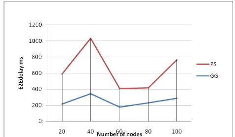
, i=1...N without relay nodes. Gain in MinMax or relay nodes impact is significant for sparsely deployed nodes. It has also computed the throughput and end-to-end delay for both cases and plotted the graphs at figure.11 & figure.12. Increase in end-to-end delay and decrease in throughput is implied due to increased hops in the communication. Since the objective is to reduce power consumption and increase in network life time, the variations in throughput and end-to-end delay are acceptable.
5.
CONCLSION
As shown explained in the previous section, the proposed PS algorithm has clearly established improvement in MinMax, MinToatl, InterAvg and InterMax terms. However, cost of the relay nodes and increased end-to-end delay to be traded with the saving obtained in the above specified aspects. In the present study, the additional nodes are placed on Euclidean line to connect the unconnected nodes. However, further optimizations are also possible by position the additional nodes at optimal places.
PS Algorithm
Input: Set of
V
nodes eachv
V
and each node is powered with lowest normalized powerp
1.
G
(
V
,
E
)
with all nodes configured withlowest normalized power
p
.G
is not connected graph2.
G
ps
(
V
ps,
E
ps)
is a connected graph with lowest normalized powerp
3.
G
(
V
,
E
)
4.
V
ps
5.
E
ps
6.
G
ps
(
V
ps,
E
ps)
7. for all
v
V
do8.
V
ps
V
ps
v
9. end for
10. for all
e
(
u
,
v
)
E
do11. if
v
u
and(
u
,
v
)
p
and(
v
,
u
)
p
then12.
E
ps
E
ps
{
e
}
13.E
E
\
{
e
}
16. While
G
psis not a connected graph do17.
e
min{(
u
,
v
)
E
,
|
u
,
v
|
p
}
18.
N
{(|
u
,
v
|
1
)
/
p
}
1
19.
N
u
,
v
/
N
20. fori
1
toN
21.
u
i
locationu
N
inu
,
v
direction22.
Vps
u
i23.
e
(
u
,
u
1)
or(
u
i,
u
i1)
or(
u
N,
v
)
as case may be24.
E
ps
E
ps
{
e
}
25.
G
ps
(
V
ps,
E
ps)
26. end for
27.
E
E
\
{
e
}
28. end while
29. while unprocessed
e
(
u
,
v
)
whereps
V
u
(
andu
V
or(
v
V
psand
V
v
or(
u
,
v
V
)
do30.
G
'
ps
G
ps\
{
e
}
31. if
G
'
ps
connectedG
(
V
,
E
)
then32.
G
ps
G
'
ps33. end if 34. end while
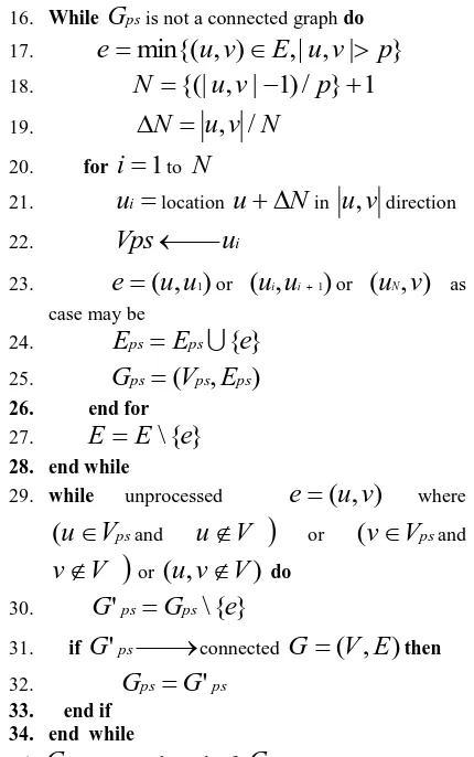
[image:5.595.68.283.72.415.2]Output:
G
psconnected graph ofG
Figure-5 PS-Algorithm
0 0.2 0.4 0.6 0.8 1 1.2
20 40 60 80 100
M
in
M
ax
number of nodes
PS
GG
RNG
LMST
OTC
OTTC
XTC
[image:5.595.315.551.72.211.2]FLSS
[image:5.595.65.573.390.660.2]Figure.6a Comparison of MinMax for different algorithms
Figure 6b. Comparison of MinMax with and without relay nodes
0 10 20 30 40 50 60
20 40 60 80 100
M
inTot
al
number of nodes
PS GG RNG LMST OTC OTTC XTC FLSS
Figure7. Comparison of MinTotal for different algorithms
0 20 40 60 80 100 120
20 40 60 80 100
In
et
rM
ax
Number of nodes
PS
GG
RNG
LMST
OTC
OTTC
XTC
FLSS
0 20 40 60 80 100
20 40 60 80 100
Number of nodes
In
te
rA
vg
PS GG RNG LMST OTC OTTC XTC FLSS
Figure9. Comparison of InterAvg for different algorithms
0 5 10 15 20 25 30
20 40 60 80 100
Network size
N
u
m
b
e
r o
f r
e
la
y n
o
d
e
s
[image:6.595.312.551.71.210.2]0.1 0.2 0.3
Figure 10. Number of relay nodes with different transmit power levels
Figure 11. Comparison of throughput with and without relay nodes
[image:6.595.313.550.76.341.2]Figure 12. Comparison of end-2-end delay with and without relay nodes
Figure 13 Network life time comparison with and without relay nodes
6.
REFERENCES
[1] M. Cardei, J.Wu, and S.Yang, ”Topology control in ad-hoc wireless networks using cooperative communication”, IEEE Transactions on Mobile computing, vol.5, no.6, pp 711-724, 2006
[2] Kenji Miyao, Hidehia nakayama, Nirwan Ansari, and Nei Kato, “LTRT: An efficient and reliable topology control algorithm for ad-hoc networks”, IEEE Transactions onwireless communications, vol.8, no.12, pp 6050-6058 Dec 2009
[3] Renato E.N.Moraes, Celso C. Ribeiro, and Christophe Duhamel, “Optimal Solutions for Fault-Tolerent Topology Control in Wireless Ad-hoc network”, IEEE Transactions on wireless communications”, vol.8, no.12, pp 5970-5981, Dec 2009
[4] M.A.Rajan , M.Girish Chandra , Lokanatha C. Reddy, and Prakash S. Hiremath, “Topological and Energy Analysis of K– Connected MANETs: A Semi-Analytical Approach”, IJCSNS International Journal of Computer Science and Network Security, VOL.8 No.2, February pp199-206
[5] Xinhua Liu, Fangmin Li and Hailan Kuang, “An Optimal Power-controlled Topology Control for Wireless Sensor Networks”, Proc. International Conference on Computer Science and Software Engineering, 2008, pp 550-554 [6] Niranjan Kumar Raya and Ashok Kumar Turuka,
“Analysis of topology control alorithms in ad-hoc and sensor networks”, Proc. International conference on challenges and applications of mathematics in science and technology (CAMIST), pp 562-571, Jan 2010 [7] Chen Wei et al, “AsOR: An Energy Efficient Multi-Hop
[image:6.595.67.287.279.402.2]Transactions on wirless communications, vol-8, no-5, May, 2009
[8] Jonathan L.Bredin, Erik D.Demaine, Mohammad Taghi Hajiaghayi, and Daniela Rus, “Deploying Sensor Networks with guaranteed fault tolerance”, IEEE/ACM Transactions on networking, vol-18,no-1, February 2010 [9] Martin Bhurkhart, Pascal von Rickenbanch, Roger
Wattenhofer, Aaron Zollinger, “Does topology control reduce interference?” MobiHoc’04, May 24-26, 2004, Roppongi, Japan.
[10]G.Xing, C.Lu, Y.Zhang, Q.Huang, and R.Pless, “Minimum power configuration for wireless communication in sensor networks”, ACM Transactions, Sensor networks, vol.3, pp200-233, 2007 [11]R.Madan and S.Lall, “” Distributed algorithms for
maximum lifetime routing in wireless sensor networks”, IEEE Transactions Wireless Communications vol.5 pp 2185-2193, 2006
[12]M.K.Maria and S.R.Das, “On-demand multipath distance vector routing in ad-hoc networks”, Proceedings 9th International Conference Network Protocols, Revierside, pp 14-23, 2001
[13]L.Lazos, andR.Poovendran, “SeRLoc: secure range-independent localization for wireless sensor networks”,in Proc. ACM WiSe ’04, 2004pp 21-30 [14]A. Caruso, S. Chessa, S.de, and A.Urpi, “GPS free
coordinate assignment and routing in wireless sensor networks”, Proc. IEEE INFOCOMM 2005, vol .1, pp 150-160 Mar 2005
[15]Ramanathan R and Redi J, “A Brief Overview of Ad Hoc Networks: Challenges and Directions,” IEEE communication magazine, pp. 20-21, May 2002. [16]L. Kirousis, E. Kranakis, D. Krizanc and A. Pelc, "Power
Consumption in Packet Radio Networks”, Theoretical Computer Science, pp. 289 - 305, 2000.
[17]G.Toussiant, The relative neighborhood graph of finite planar set, Pattern Recognition 12(4) (1980) 61-268 [18]K.R.Gabriel, R.R.Sokal, A new statistical approach to
geographic variation analysis, Systematic zoology 18 (1969) 259-278
[19]Ning Li, Localized topology control in wireless networks, PhD thesis, 2005
[20]D.M.Blough, M.Leoncini, G.Resta, and P.Santi,”On the symmetric range assignment problem in wireless ad hoc networks”, in Proc. 2nd
IFIP International conference onTCS, 2002, pp 71-82
[21]G.Calinescu, I.L.Mandoiu, and A.Zelikovsky, “Symmetricconnectivity with minimum power consumption in radio networks”, Proc. 17th IFIP World
Comput. Congress, 2002 pp 119-130
[22]L.M.Kirousis, E.Kranakis,D.Krizanc, and A.Pelc, “Power consumption in packet radionetworks”, Theoretical Computer Science, vol-243, no:1-2, 2000, pp 289-305
[23]V.kawadia, P.Kumar, “Power control and clustering in ad hoc networks”, Proc of IEEE Infocom, San Francisco, CA, 2003, pp. 459-469
[24]L.Li, J.Y.Halpern, P.Bahl,Y.Wang, and R.Wattenhofer,”Analysis of a cone-based distributedtopology control algorithm for wireless multi-hop networks”, in Proc. ACM PODC 2001,Aug. 2001, pp 264-273
[25]J. Cartigny, D. Simplot, and I.Stojmenovic, “Localized Minimum energy broadcasting in ad-hoc networks”, in Proc. IEEE INFOCOMM 2003, vol.3, March 2003,pp 2210-2217
[26]N.Li, J.Hou, C.Sha,and L.Sha, “Design and analysis of anMST-based topology control algorithm”, IEEE Transactions on wireless communications”,vol.4, no.3, pp 1195-1206, May, 2005
[27]R.Komali, A.MacKenzie, and R.Gilles, “Effect of selfish node behavior on efficient topology design”, IEEE Transactions on Mobile computing, vol.7, no.9, pp 1057-1070, sep 2008
[28]Kevin Chan , Ananthram Swami , Qing Zhao , and Anna Scaglione, “CONSENSUS ALGORITHMS OVER FADING CHANNELS “,The 2010 Military Communications Conference - Unclassified Program - Netw orking Protocols and Performance Track
7. AUTHORS PROFILE
B.Brahma Reddy obtained his B.Tech from JNTU and M.Tech from IIT, Madras in 1980 & 1982 respectively. He has worked for Indian Institute of Science, Indian Telephone Industries, National Informatics Centre, DishnetDSL, Reliance Infocomm for nearly 25 years. Past 6 years he is working as Professor in JNTU affiliated college. Currently he is perusing his Doctoral programme.