Ant-Colony-based Algorithm for Multi-Target Tracking in
Mobile Sensor Networks
S.Barath Kumar
PG Scholar/ECE Department
Sri Shakthi Institute of Engineering and Technology Coimbatore, India
G.Myilsamy
Assistant Professor / ECE Department Sri Shakthi Institute of Engineering and Technology
Coimbatore, India
ABSTRACT
Target tracking is one of the applications of Mobile Sensor Networks. Mobility management is the important parameter that affects the performance and lifetime of the Mobile sensor networks. So we need to manage the mobility in a controlled manner. Existing methods attempt to achieve these requirements for controlled mobility single target tracking only. In this paper, we propose a Multi-Target Tracking method using Ant Colony Optimization to satisfy these requirements. In this proposed method, targets current position values are estimated at every time step. Then, predicting the next position value of each target by using the previous time-step estimated values. Interval Analysis is used for estimation and prediction of position values. Then the proposed method consists of moving the mobile node in an optimal way to cover Multi-Target. The optimal path is been chosen by Ant Colony Optimization technique. Simulations results shows the advantages of the proposed method compared to single target tracking methods.
General Terms
Swarm Intelligence, Optimization Techniques, Wireless Communications.
Keywords
Ant colony, Controlled Mobility, Interval Analysis, Mobile Sensor Network, Multi-Target Tracking.
1.
INTRODUCTION
Mobile sensor networks (MSN) have significant impact upon the efficiency of military and civil applications such as environment monitoring, target surveillance, industrial process observation, tactical systems, etc, [1]. In these scenarios, target tracking is one of the most important applications of mobile sensor networks [2]. MSN contains element like processor, sensor, transceiver, battery and movement capabilities. Mobility may be of active or passive. In the active type, sensors are moved in a controlled manner. Passive mobility will not have any control, it will move in some random manner. It is very difficult to manage passive mobility, so in this proposed method, controlled mobility is used.
Target tracking using a sensor network was initially investigated in 2002 [3]. In a given field of surveillance interest, there are varying numbers of targets. They arise in the field at random locations and at random times. The movement of each target follows an arbitrary but continuous path, and it persists for a random amount of time before disappearing in the field. The target locations are sampled at random intervals. The goal of the Multi-Target Tracking (MTT) problem is to find the moving path for each target in
the field [3]. To the best of our knowledge, the idea of using a particle filter for a binary sensor network approach has been first proposed in [4] for target tracking application. However, most of the work related to binary sensing has been applied to the case of tracking a single target only [5]. In [6], [7], particle filtering algorithms for target tracking using quantized data in Wireless Sensor Networks have been proposed, however wireless channel imperfections have not been considered as part of the tracking problem. There are some schemes developed for controlled mobility: DARA [8] e-PADRA [9]. These algorithms restore network connectivity through controlled relocation of movable nodes. But in these schemes, optimal placement of the nodes is too expensive and also it is impossible for different environmental implementation. In [10], authors proposed a method to manage the mobility of the nodes based on Bayesian estimation theory. This method is suited only for networks when the target and sensor nodes are moves with constant velocities.
This paper consists of three important processes which is been iterative at each time step. At first, the current position value of the targets are been estimated. Then the next position value is been predicted by current and previous positions estimates. In the final process, a set of new predicted values of the multi-target are there, so sensor is moved in an optimal way to cover these targets. This could be done by Ant Colony Optimization technique where each mobile node is assigned one new location within the computed set.
The estimation phase and the prediction phase are computed using interval analysis [11]. Our deployment area is of rectangular field so two-dimensional intervals are used to find the estimation and prediction phases. ACO algorithms have been applied to many combinatorial optimization problems, ranging from routing vehicles, stochastic problems, multi-targets, travelling salesman problem and parallel implementations [12].
The rest of the paper is organized as follows: In Sections 2, we describe the determination of targets current position and the basics of Interval analysis. In section 3, prediction of targets next step position values by using the prediction models is dealt. Section 4 describes about the Ant Colony Optimization technique and its algorithm. Simulation results are given in Section 5. Section 6 concludes the paper
2.
DETERMINATION OF TARGETS
CURRENT POSITION
2.1
Interval Analysis
The Interval analysis represents a rigorous mathematical tool aiming at manipulating intervals instead of real numbers [13]. A real interval x is a nonempty set of real numbers.
(1) where and are called the infimum and the supremum values respectively. The interval could also be defined by its centre C([x]) = ( + )/2, and width W([x]) = - .
A multidimensional interval of IRn, also called box, is given by the cartesian product of n real intervals as follows:
[x] = [x1] x……. x [xn] (2) Standard set operations are naturally defined on intervals, such as equality (=), inclusion (⊂), intersection (∩) and convex union defined as:
[x] [y] = [min{ , }, max{ , }] (3)
Arithmetic operations are also extended to intervals. For instance, we list the following basic operations,
[x] + [y] = [ + , + ]; [x] - [y] = [ - , - ] (4) The arithmetic operations on intervals may take advantage of some algebraic properties such as associativity, commutativity and distributivity.
2.2
Problem Statement
Every node cannot be always active in sensing. In this method, each sensor node detects one bit of information from the target. This one bit could be used to indicate whether the target is within the sensor range or moving away from the sensor range. Now consider the sensing range be a circular disk having r as radius. According to the Okumura-Hata model, the power of a signal decreases with the increase of the distance travelled by this signal [14]. If the target is active and communicating with the sensor, assume that all these signals are emitted with the same initial power. Let P(r) be the power of a target signal corresponding to a travelled distance equal to r. Then, sensor nodes receiving target signals with powers P larger than P(r) are located at distances to the target less than r is shown in Fig.1.
Fig. 1 Sensing Range of Sensor
We know that the distance between the target and the sensor is less than r. So we can calculate the current position value by solving this distance equation:
(y1(t) - xi,1 (t)) 2
+ (y2(t) – xi,2(t)) 2 ≤ r2
, (5) where (y1(t), y2(t)) be the co-ordinates of the unknown position of the target and x be the co-ordinate position of ith sensor.
[image:2.595.65.259.692.750.2]All the position parameters are considered as two-dimensional interval box 2D. Our deployment area is a rectangular field. The entire area is been divided into many row and columns. This defines a particular box for a respective row and column [15]. So this two dimensional box is used as a field area in which the estimation of the current position of the Target is been confined to particular boxes. An example is shown in Fig. 2
Fig. 2 Example of 2D Box of size 4x4
Our work is now reduced to find the minimal box that contains all possible locations. Let us consider the distance equation in interval frame work:
[[y1](t)-xi,1 (t)]2 + [[y2](t) – xi,2(t)]2 ≤ [0, r2] (6) where [y](t) = [y1](t) x [y2](t) is the Target boxed position at time t. This problem is called as Constraint satisfaction problem where the large area is been contradicted to the smallest box.
2.3
Waltz Algorithm
The algorithm used for contraction is called Waltz contractor algorithm. It is a forward-backward algorithm that iterates over all constraint [16]. Equation (6) can yields two expressions in which one co-ordinate is expressed in terms of other that iterates each time step
[y1](t) [yi,1(t) - i,1 , xi,1(t) + i,1]
[y2](t) [yi,2(t) - i,2 , xi,2(t) + i,2] (7) where – and
– .The above equation (7) is iterated using the Waltz algorithm. It is a forward-backward algorithm that iterates over all constraint. The algorithm is
Algorithm 1: Estimation algorithm
Input: Indices of sensors observing the Target; Output: Target coordinates [y1](t) and [y2](t); Initialization: [y1](t) = [Y1], [y2](t) = [Y2], A = W([y1]).W([y2]), Aold = A+1; While A < Aold do
Aold = A; for i ϵ I do
i, – ; [y1](t) = [y1](t) ∩ [xi,1(t) - i,1 , xi,1(t) + i,1] ;
– ; [y2](t) = [y2](t) ∩ [xi,2(t) - i,2 , xi,2(t) + i,2] ;
end
A = W([y1]).W([y2]); end
The Waltz algorithm is used for the estimation phase using the interval analysis method. This algorithm is iterated for each time for all the sensors.
3.
PREDICTION OF NEXT POSITION
Once the positions of the Targets are been estimated, then the next step position of the Target is been predicted. This is done by the joint support of kth order prediction model and instant velocity and acceleration model. In MSNs each Target is moving at different velocities so this combine support of these methods will improve the accuracy.
Let y( ),y(2),…….,y(t) be all available estimated position of the Target. All the y variables are of 2D because from the estimation phase we used 2D Interval based algorithms [13]. Then, a kth order prediction model is given as follows:
1 (t + 1) = f(y1(t) , y1(t-1),. . . , y1(t – k)),
1 (t + 1) = f(y1(t), y1 (t-1), y1(t-2));
2 (t + 1) = f(y2(t), y2 (t-1), y2(t-2)) (9) According to Newton's second law of motion. The 2nd order prediction formula is formulated as follows:
(t+1) = y (t) + t.u(t) + . (t), (10) where Δt-time interval between two successive time steps and u(t) and a(t) are the respective instant velocity and instant acceleration and it is given by
(11)
(12) where u(t) and a(t) are the values which have relation with motion of the Targets. Here an important note is the term u(t-1) holds the value of y(t-2) estimated value. In the interval framework, the prediction model is formulated as follows:
[ (t + 1)] = [y(t)] + t.[u(t)] + .[a(t)], (13) where [ (t + 1)] is the predicted position box of the Target, equation (12) can be used for 2D interval based algorithms to obtain value of y1 and y2. Likewise for the velocity and acceleration, the interval formula’s are given by
(14)
(15) From equation (13) we can calculate the next-step position for each target at every time step.
4.
ANT COLONY OPTIMIZATION
ALGORITHM
The Ant Colony Optimization algorithm (ACO) is a probabilistic technique for solving computational problems. It is based on the behaviour of ants seeking a path between their colony and a source of food. In the natural world, ants (initially) wander randomly, and upon finding food return to their colony while laying down pheromone trails. If other ants find such a path, they are likely not to keep travelling at random, but to instead follow the trail [17]. Over time, however, the pheromone trail starts to evaporate, thus reducing its attractive strength. The more time it takes for an ant to travel down the path and back again, the more time the pheromones have to evaporate. In this way, ants can search for the shortest path from their nest to a food source with only pheromone information.
The process contains three main steps and their diagram also shown below in Fig. 3:
1.The first ant finds the food source F, via any way a, then returns to the nest N, leaving behind a trail pheromone b. 2.Ants indiscriminately follow four possible ways, but the
strengthening of the runway makes it more attractive as the shortest route.
3.Ants take the shortest route; long portions of other ways lose their trail pheromones.
ACO was aimed to solve the Travelling Salesman Problem [18], in which the goal is to find the shortest path that traverses all cities exactly once and then returns to the starting city. Let us consider, there are N cities and the total number of ants is M. Each ant chooses the next city with a probability in accordance with the distance between the current city and the next city and in accordance with the intensity of the pheromone [19]. At each iteration of the algorithm, each ant moves from state i to state j, then the transition probability for the k-th ant is given by
pkxy =
kxy xy
xy xy α
)
)(
(
)
)(
(
(16)
where
xy is the amount of pheromone deposited for transition from state x to y,
xy is the desirability of state transition x to y and it is defined as
xy
1
/
d
xy , where dxy is the Eucliean distance between state x and state y. The parameters α and β are the constants used to control the influence of the variable.
Fig. 3 Concept of Ant Colony Optimization (Food Source-F, Nest-N, Any way-a and Trail way-b)
Once all the ants have completed a solution, then the trails should be updated by the formula:
xy k
xy k xy
xy
(
1
)
(17)where ρ is the pheromone evaporation coefficient or also called as local pheromone decay parameter typically takes value between 0 to 1 and
kxy is the amount of pheromonedeposited by k-th ant , the value is given by,
kxy=Q/Lk ; if k-th ant uses edge (x,y) in its tour, otherwise the value is zero .So in this ACO approach, the greater the probability that edge will be chosen. This process is being done iterative once the termination conditions are satisfied. Then the best path will be obtained by this method. This path is used for moving the sensor in an optimal way.
5.
SIMULATIONS
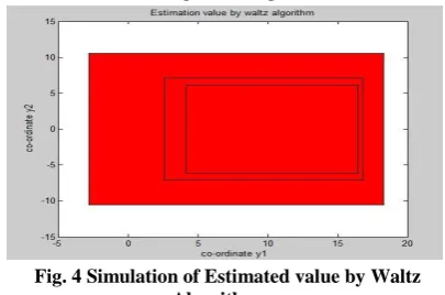
In this section, we will describe our simulation environment and some experimental results from the algorithm we stated. All simulations were on a PC with an Intel Core i5 CPU 760 operating at 2.80GHz, 4GB of RAM using MATLAB 7.9. We implemented the INTLAB 6 toolbox in the MATLAB for Interval Analysis. For example consider the deployment area of size 16 X 16m2. Then the number of Targets in the field are three per sensor. Sensor initial location is given by the interval (3,2) in the co-ordinate box. Then by the waltz algorithm, the estimated value of the target is minimal box solution that contains all possible solutions. The estimated minimal box is shown in the Fig.4.
For the prediction of new position value, we used second order prediction model k=2 and the time interval between two successive steps is Δt=0.05 seconds. These specification parameters are used in this prediction phase.
[image:3.595.330.533.624.758.2]
Let us consider the sensor previous locations are (3,2), (2,3) and (4,1). Then the predicted value obtained is y1 is 6 and y2 is 11. This is shown in the Fig.5 by (exp1, exp2) value.
[image:4.595.66.262.102.254.2]
Fig. 5 Result of Predicted value by current and previous position estimates.
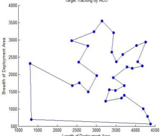
In the optimization phase, the area of interest is been defined temporarily as 4500 x 4500 m2. Let us consider the number of ants is lower than the number of cities (M<N). Number of cities consider is N=100, the number of ants used is M=31, the pheromone decay parameter value is ρ=0.5 and the constant parameters values are taken as α= , β=5 and Q = 00. The simulation for this scenario is shown in Fig.6. We can improve the result by varying the constant parameters value. As per the result of prediction values, the ACO chooses the best path in order to cover the multi-targets.
[image:4.595.79.257.375.532.2]
Fig. 6 Result of simulation when number of Ants is M=31 and number of Cities is N=100
Let us consider another scenario where number of ants is higher than the number of cities (M>N) where M=150 and N= 00. The constant parameters values are taken as α =2, β =4 and Q =100.
Fig. 7 Result of simulation number of Ants is M=150 and number of Cities is N=100
There are some criteria is there to choose the value of parameters α and β where α ≥ 0 and β ≥ . And we know that the value of ρ range from 0 to . The simulation for this specification is shown in Fig.7.
From the two scenarios, it is known that we can obtain better results by varying the constant parameters and the pheromone decay parameter ρ.
6.
CONCLUSIONS
This paper proposed a method for Multi-Target Tracking in Mobile Sensor Networks. This method consists of estimating the current position of the target and then predicting its following position using a second-order prediction model and Instant Velocity and Acceleration relation. Estimation and Prediction are been done by the Interval Analysis method, where target positions are boxed. Then prediction phase gives a set of candidate position. The optimal path travelled to cover the Multi-Target is done by using the Ant Colony Optimization algorithm. The proposed approach uses the mobile nodes. Simulation results illustrate the advantages of the proposed method compared to single Target Tracking methods developed for static sensor networks.
7.
REFERENCES
[1] G. Song, Y. Zhou, F. Ding, and A. Song, “A Mobile Sensor Network System for Monitoring of Unfriendly Environments,” Sensors, vol. 8, pp. 7259-7274, Nov. 2008.
[2] Sunita, Jyoti Malik and Suman Mor, “Comprehensive Study of Applications of Wireless Sensor Network”, International Journal of Advanced Research in Computer science, vol.2, Issue.11,Nov.2012.
[3] T.P. Lambrou, C.G. Panayiotou, S. Felici, and B. Beferull, “Exploiting Mobility for Efficient Coverage in Sparse Wireless Sensor Networks,” Wireless Personal Comm., vol. 54, no. 1, pp. 187-201, Apr. 2009.
[4] J. Aslam, Z. Butler, V. Crespi, G. Cybenko, and D. Rus, “Tracking a moving object with a binary sensor network”, Proc. ACM Int. Conf. Embedded Networked Sensor Systems SenSys, 2003.
[5] Shrivastava.N, Mudumbai.R, Madhow.U, and Suri.S, “Target tracking with binary proximity sensors: Fundamental limits, minimal descriptions, and algorithms”. In Proc. of ACM, SenSys, 2009.
[6] Y. Ruan, P. Willett, A. Marrs, F. Palmieri, and S. Marano, “Practical fusion of quantized measurements via particle filtering,” IEEE Trans. Aerosp. Electron. Syst., vol. 44, no. 1, pp. 15–29, Jan. 2008.
[7] L. Zuo, R. Niu, and P. K. Varshney, “A sensor selection approach for target tracking in sensor networks with quantized measurements,” in Proc. Int. Conf. Acoustics, Speech, and Signal Processing (ICASSP), Las Vegas, NV, Apr. 2008.
[8] A. A. Abbasi, M. Younis and K. Akkaya, “Movement-Assisted Connectivity Restoration in Wireless Sensor and Actor Networks,” in IEEE Transactions on Parallel and Distributed Systems, Volume 20 Issue 9, September 2009.
[image:4.595.84.250.603.738.2]Mobility,” in IEEE Trans. on Computers, vol. 59, no. 2, pp. 258-271, Feb. 2010.
[10]Y. Zou and K. Chakrabarty, “Distributed Mobility Management for Target Tracking in Mobile Sensor Networks,” IEEE Trans. Mobile Computing, vol. 6, no. 8, pp. 872-887, Aug. 2007.
[11]A. Gning, L. Mihaylova, and F. Abdallah, “Mixture of uniform probability density functions for non linear state estimation using interval analysis,” in Proc. of the International Conf. on Information Fusion, Edinburgh, UK, 2010.
[12]J.W. Lee, B.S. Choi, and J.J. Lee, ”Energy-Efficient Coverage of Wireless Sensor Networks Using Ant Colony Optimization with Three Types of Pheromones”, IEEE Transactions on Industrial Informatics, Vol.7, No. 3, Aug. 2011, pp. 419-427.
[13]R.E. Moore, R. Baker Kearfott and M.J. Cloud, “Introduction to Interval Analysis”, Society for Industrial and Applied Mathematics, 2008.
[14]Z. Nadir, N. Elfadhil, and F. Touati, “Pathloss Determination Using Okumura-Hata Model and Spline Interpolation for Missing Data for Oman,” Proc. World Congress Eng., vol. 1, July 2008.
[15]Abdallah. F, Gning .A and Bonnifait, “Box Particle Filtering for non Linear State Estimation using Interval Analysis. Automatica, volume 44, pp. 807-815, 2008. [16]F. Mourad, H. Snoussi, F. Abdallah, and C. Richard,
“Guaranteed Boxed Localization in MANETs by Interval Analysis and Constraints Propagation Techniques,” Proc. IEEE GlobeCom, 2008.
[17]Zhibin Xue1, Jianchao Zeng, Caili Feng, and Zhen Liu “Swarm Target Tracking Collective Behavior Control with Formation Coverage Search Agents & Globally Asymptotically Stable Analysis of Stochastic Swarm” Journal of Computers, vol. 6, no. 8, August 2011. [18]M. Dorigo and L. M. Gambardella, “Ant Colony System:
A Cooperative Learning Approach to the Travelling Salesman Problem”, IEEE Transactions on Evolutionary Computation, Vol. 1, No. 1, Apr.1997, pp. 53-66. [19]Joon-Woo Lee, Ju-Jang Lee, Ant-Colony-Based