Generalized maximum entropy (GME) estimator: formulation and a monte carlo study

Munich Personal RePEc Archive

Generalized maximum entropy (GME)

estimator: formulation and a monte carlo

study

Eruygur, H. Ozan

26 May 2005

Online at

https://mpra.ub.uni-muenchen.de/12459/

Paper presented at the

VII. National Symposium on Econometrics and Statistics Istanbul, Turkey, May 26-27, 2005

GENERALIZED MAXIMUM ENTROPY (GME)

ESTIMATOR: FORMULATION AND A MONTE

CARLO STUDY

H. Ozan ERUYGUR

Middle East Technical University Department of Economics

Ankara 06531 Turkey

[email protected]

ÖZET

Entropinin kökeni 19. yüzyıla kadar uzanır. Belirsizlik ölçütü olarak geliştirilmesi ise Shannon (1948) tarafından olmuştur. Yaklaşık 10 yıl sonra 1957’de Jaynes, Shannon’un entropisini özellikle kötü tanımlanmış problemler için bir tahmin ve çıkarım methodu olarak Maksimum Entropi (ME) ilkesi adıyla formüle etmiştir. Yakın tarihte, Golan et al. (1996) Genelleştirilmiş Maksimum Entropi (GME) tahmincisini geliştirerek yeni bir tartışmayı başlatmıştır. Bu yazı

iki kısımdan oluşmaktadır. İlk kısım, bu yeni tekniğin (GME) formülasyonu üzerinedir. İkinci kısımda ise bir Monte Carlo çalışmasıyla normal dağılmayan hata terimleri durumunda GME’nin tahmin sonuçları tartışılacaktır.

Anahtar Kelimeler: Entropi, Maksimum Entropi, ME, Genelleştirilmiş Maksimum Entropi, GME, Monte Carlo, Shannon Entropisi, Normal dağılmayan hata terimi.

ABSTRACT

The origin of entropy dates back to 19th century. In 1948, the entropy concept as a measure of uncertainty was developed by Shannon. A decade after in 1957, Jaynes formulated Shannon’s entropy as a method for estimation and inference particularly for ill-posed problems by proposing the so called Maximum Entropy (ME) principle. More recently, Golan et al. (1996) developed the Generalized Maximum Entropy (GME) estimator and started a new discussion in econometrics. This paper is divided into two parts. The first part considers the formulation of this new technique (GME). Second, by Monte Carlo simulations the estimation results of GME will be discussed in the context of non-normal disturbances.

I. INTRODUCTION

The origin of entropy dates back to 19th century. In 1948, the entropy concept as a measure of uncertainty (state of knowledge) was developed by Shannon in the context of communication theory. A decade after in 1957, E. T. Jaynes formulated Shannon’s entropy as a method for estimation and inference particularly for ill-posed problems by proposing the so called Maximum Entropy (ME) principle. More recently, Golan et al. (1996) developed the Generalized Maximum Entropy (GME) estimator and started a new discussion in econometrics.

Our paper is divided into two parts. The first part considers the formulation of this new technique of Generalized Maximum Entropy (GME). In the second part, by performing Monte Carlo simulations, we will discuss the estimation results of GME in the case of non-normal distributed disturbances.

II. THE GENERALIZED MAXIMUM ENTROPY APPROACH

Suppose that we observe a T-dimensional vector y of noisy indirect observations on an unknown and unobservable K-dimensional parameter vector β, where y and β are related through the following linear model relationship

y=Xβ+u (EQ.1)

where X is the TxK known matrix of explanatory variables and u is a Tx1 noise (disturbance) vector.

In order to be able to use Jaynes’ Maximum Entropy principle for the estimation of regression parameters, the parameters β must be written in terms of probabilities because of the fact that the arguments of the Shannon’s maximum entropy functionI are probabilities.

zkm, as the possible realizations of βk with corresponding probabilities pkm, we can convert

each parameter βk as follows:

1 M

k km km m

z p

β

=

=

∑

Let us define the M dimensional vector of equally distanced discrete points (support space) as

′_k

z =[zk1, zk2,…, zkM] and associated M dimensional vector of probabilities as pk=[pk1, pk2,…,

pkM]′. Now, we can rewrite β in (EQ.1) as

β= Zp=

0 . 0 0 . .

. . . 0 . 0 . 0

′ ⎡ ⎤ ⎡ ⎤ ⎢ _′ ⎥ ⎢ ⎥ ⎢ ⎥ ⎢ ⎥ ⎢ ⎥ ⎢ ⎥ ⎢ _′ ⎥ ⎢ ⎥ ⎣ ⎦ ⎣ ⎦ 1 1 2 2 K K z p z p z p (EQ.3)

where Z is a block diagonalKxKM matrix of support points with

/

k k

z p =

1 M

km km k m

z p β

=

=

∑

where pk is a M dimensional proper probability vectorII corresponding to a M dimensional

vector of weights zk. Recall that the last vector, zk, defines the support space of βk. By this

way, each parameter is converted from the real line into a well-behaved set of proper probabilities defined over the supports.

As can be seen, the implementation of the maximum entropy formalism allowing for

unconstrained parameters starts by choosing a set of discrete points by researcher based on his a priori information about the value of parameters to be estimated, where these set of discrete points are called the support space for all parameters. In most cases, where researchers are uninformed as to the sign and magnitude of the unknown βk, they should

magnitude, say z′_k=[-C, -C/2, 0, C/2, C] for M=5 and for some scalar C [Golan et al., 1996:77].

Similarly, we can also transform the noisesu as follows [Golan et al., 1996:87]:

1 J t tj tj

j

u v w

=

=

∑

Notice that by this conversation, Golan et al. (1996:121) propose a transformation of the possible outcomes for ut to the interval [0,1] by defining a set of discrete support points

′ t

v =[vt1, vt2,…, vtJ] which is distributed uniformly and evenly around zero (such that vt1=-vtJ

for each t if we assume that the error distribution is symmetric and centered about 0)III and a vector of corresponding unknown probabilities wt=[wt1, wt2,…, wtJ]′ where J≥2. Now, we can

rewrite u in (EQ.1) as

u= Vw =

0 . 0 0 . .

. . . 0 . 0 . 0

′ ⎡ ⎤ ⎡ ⎤ ⎢ _′ ⎥ ⎢ ⎥ ⎢ ⎥ ⎢ ⎥ ⎢ ⎥ ⎢ ⎥ ⎢ _′ ⎥ ⎢ ⎥ ⎣ ⎦ ⎣ ⎦ 1 1 2 2 T T v w v w v w (EQ.6) with / t t

v w =

1 J

tj tj t j

v w u

=

=

∑

In (EQ.4) and (EQ.7) the support spaces zk and vt are chosen to span the relevant parameter

spaces for each {βk} and {ut}, respectively. As for the determination of support bounds for

disturbances, Golan et al (1996) recommend using the “three-sigma rule” of Pukelsheim (1994) to establish bounds on the error components: the lower bound is vL = -3σy and the

upper bound is vU = 3σy, where σy is the (empirical) standard deviation of the sample y. For

Under this reparameterization, the inverse problem with noise given in (EQ.1) may be rewritten as

y=Xβ+u = XZp +Vw (EQ.8)

Jaynes (1957) demonstrates that entropy is additive for independent sources of uncertainty. The details of this property can be found in Kapur and Kesavan (1992:31-32). Therefore, assuming the unknown weights on the parameter and the noise supports for the linear regression model are independent, we can jointly recover the unknown parameters and disturbances (noises or errors) by solving the constrained optimization problem of max H(p,w)=-p′lnp-w′lnw subject to y=XZp+Vw.

Hence, given the reparameterization in (EQ.8) where {βk} and {ut} are transformed to have

the properties of probabilities, in scalar notation the GME formulation for a noisy inverse problem may be stated as

1 1 1 1

max ( , ) .ln .ln

K M T J

km km tj tj

k m t j

H p p w w

= = = =

= −

∑∑

∑∑

p,w p w (EQ.9)

subject to the constraints

1 1 1

K M J

tk km km tj tj t

k m j

x z p w v y

= = =

+ =

∑∑

∑

1 1 M km m p = =

∑

1 1 J tj j w = =

∑

where (EQ.10) is the data (or, consistency) constraint whereas (EQ.11) and (EQ.12) provide the required adding-up constraints for probability distributions of {pkm} and {wtj},

respectively.

1 1 1 ˆ ˆ ˆ T t km tk t

T t km tk t GME km M m z x z x e p e λ λ = = = − − = ∑ ∑

∑

where Ω_kp( )λˆ_t = 1

ˆ

1

T

t km tk t

M z x

m e λ = − = ∑

∑

The solution for ˆw_tj

1 ˆ ˆ ˆ t tj t tj GME tj J j v v e w e λ λ = − − =

∑

ˆ

1

ˆ

( ) tj t

J v w t t j e λ λ − =

Ω =

∑

Notice that, in the expressions above, λˆ_t represent the dual value of data constraint. Substituting the solutions of ˆp_kmand ˆw_tj into (EQ.2) and (EQ.5) produces the GME estimates of βk and ut, as

1

ˆGME M _ˆ k km km

m

p z

β

=

=

∑

and

1

ˆ ˆ

J GME

t tj tj j

u w v

=

=

∑

As can be seen, the GME estimates depend on the optimal Lagrange multipliers λˆ_tfor the

model constraints. There is no closed-from solution forλˆ_t, and hence no closed form solution

for p, w, β and u. Therefore numerical optimization techniques should be used to obtain the solutions and solutions must be found numerically.

III. A MONTE CARLO STUDY WITH NON NORMAL DISTURBANCES

distribution with unit degrees of freedom [χ2(1)] is used. Third, another chi square distribution but this time with 4 degrees of freedom [χ2(4)] is generated in order to represent a distribution which is less skewed.

For every generated data set, the model parameters are estimated with both GME and OLS and the whole procedure is repeated 1 000 times for each sample size. The sample sizes used are T=5, 10, 15, 20, 30, 40 and 50. The model estimated is a simple regression model with a constant term. The true value of the constant term is set to 0.5, while the true value of the slope parameter is set to 1.75. The econometric software Shazam 10.0 is used for the estimation of Monte Carlo trials.

The performances of the OLS and GME estimators are evaluated using the measures of absolute bias (ABIAS) and root mean square error (RMSE). Absolute bias is calculated as the absolute value of the difference between average estimate and the true value of the parameter. Root mean square error is, as known, the square root of mean square error (MSE) which is given by the sum of the squared bias and the empirical variance. The sum of all RMSE is denoted by SRMSE, and the sum of all ABIAS is denoted by SABIAS.

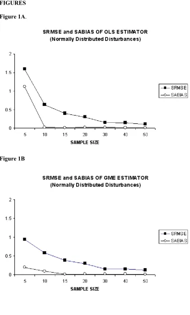
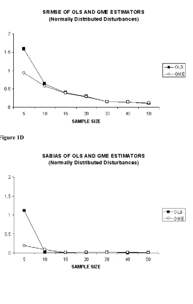
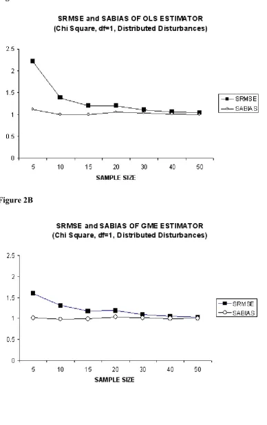
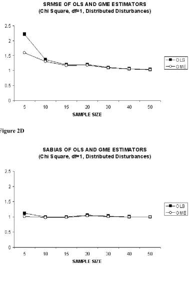
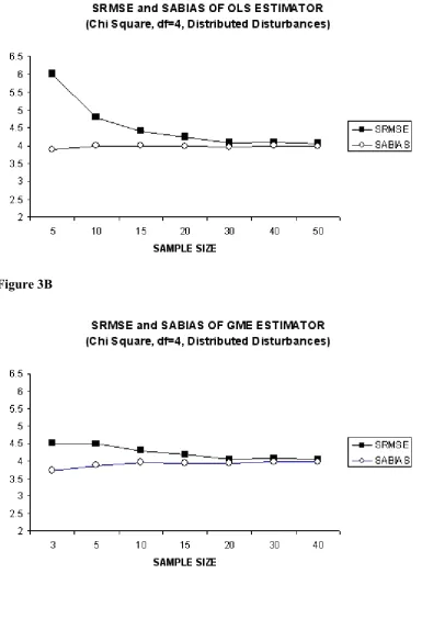
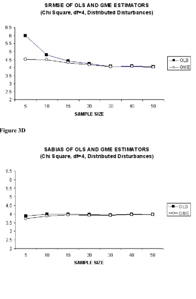
For each type of error distribution [N(0,1); χ2(1) and χ2(4)] the simulation results are presented by four figures. First figure represents the SRMSE and SABIAS of OLS estimator. Second figure shows the SRMSE and SABIAS of GME estimator. Third figure plots the SRMSE of both OLS and GME in one graph, whereas the fourth one plots the SABIAS of both OLS and GME in one graph.

such as five (T=5). Another important point that Figures 1A and 1B reveal is the fact that the behaviors of OLS and GME estimators in terms of both sum of root mean square error (SRMSE) and absolute bias (SABIAS) follow very similar patterns, starting from a sample size of fifteen (T=15). A further important point that we can note from Figures 1A and 1B is that the SRMSE of both OLS and GME estimators’ decreases with increasing sample size, which is a behavior that indicates the consistency of estimators. Note that the consistency properties of data constrained GME estimator is first established by Mittelhammer and Cardell (1997) and later developed more by Mittelhammer, Cardell and Marsh (2002). Some more details can be found in Mittelhammer R., G. Judge, and D. Miller (2000).

Recalling that the MSE is the sum of the squared bias and the empirical variance, Figure 1B shows that, while the bias represents only a small part of the RMSE, the standard errors of GME estimates constitutes the important part. For small sample sizes this could lead to poor estimates, however, this situation can be handled by including out of sample information that can be introduced into the GME estimator. In other words, the employment of some prior information would decrease the variance of estimators at small sample sizes without introducing a strong additional bias. An easy way to include such out of sample information is to use the priors on parameters or disturbance support spaces. Hence, in addition to the good performance of GME in terms of absolute bias and root mean square in small sample sizes, the root mean square error (SRMSE) can also be much more reduced by incorporating out of sample information using support spaces of parameters and disturbances. However, in this study we will not go into further details of this issue and leave it as an important topic for another study. Notice that, in this study we do not include any prior information using support spaces: support spaces are defined as zero centered symmetrically large intervals.

The large differences in absolute bias (SABIAS) of OLS and GME in small sample sizes such as five (T=5) is notable, which is the case depicted in Figure 1D. If we compare Figure 1D with figures 2D and 3D we can see that in the case of normal disturbances (Figure 1D) the absolute bias (SABIAS) of OLS is lower than that of GME, starting from a sample size of about ten (T=10). However, the same performance of OLS cannot be seen in the case of non normal disturbances (Figure 2D and Figure 3D). In these cases, the absolute bias (SABIAS) of GME is always lower than that of OLS, although this difference becomes very low after a sample size thirty (T=30). Another remarkable result form our simulation is that, with higher degrees of freedom (df=4), the absolute bias of GME is much more lower when compared to unit degrees of freedom (df=1) as depicted in Figure 2D. In addition, this behavior of the absolute bias for the GME is long lasting until a sample size of fifteen (T=15) with higher degrees of freedom when compared to unit degrees of freedom (df=1).

Consulting to Figure 2A and 3A, one can observe that SRMSE and SABIAS of OLS becomes very close to each other particularly after the sample size of thirty (T=30), whereas the same pattern is seen for GME after a sample size of only twenty (T=20). Finally, in figures 2C and 3C, SRMSE performance of GME is compared with that of OLS. When these figures are examined, the first important point to note is the highly low SRMSE of GME estimator in small sample sizes (T<15) when compared with that of OLS. As stated before, contrary to normally distributed disturbances situation, in the case of non normal disturbances the SRMSE and SABIAS of GME estimator is always lower even in large sample sizes, although the gap is very low and closes faster for low sample sizes starting from fifteen (T=15).

IV. CONCLUSION

based on the model framework of the Monte Carlo study. However, the findings are notably promising at least within the structure of our model of simulation. The findings in this paper give some clues for the use of GME estimators. First, in the case of small samples because of data unavailability, the GME estimator can give better results when compared with OLS. Second, even in the case of non normal distributed disturbances, performance of the GME estimator is good and in addition, our Monte Carlo studies show that its performance is better than normal disturbances case.

FIGURES

Figure 1A.

Figure 1C.

Figure 2A.

Figure 2C.

Figure 3A.

Figure 3C.

ENDNOTES

I

For properties of Shannon’ Entropy measure, see Kapur and Kesavan (1992:24).

II

A proper probability vector is characterized by two properties: pkm≥0, ∀ m=1,...,M and

1 1 M km m p = =

∑

Note that J≥2 points may be used to express or recover additional information about ut (e.g. skewness or kurtosis). For example if we assume that the noise distribution is skewed such that ut∼χ2(4), then

v=[− 2,2 2] can be used as support space for noise representing the skewness.

IV

One can easily show that

1 1 1 1 1

K

tk k k

K M K M

tk km km tk km km

k m k m

x β x z p x z p

= = = = =

= =

∑

∑ ∑

∑∑

REFERENCES

Jaynes, E. T. (1957). "Information Theory and Statistical Mechanics." Physics Review, 106, 620-630.

Golan, A., Judge, G. and Miller D. (1996), Maximum Entropy Econometrics: Robust Estimation With Limited Data, John Wiley & Sons.

Kapur, J.N., & Kesavan, H.K. (1992), Entropy Optimization Principles with Applications, Academic Press, London.

Mittelhammer, R. and S. Cardell (1997), “On the Consistency and Asymptotic Normality of the Data Constrained GME Estimator of the GML”, Working Paper, Washington State University, Pullman, WA.

Mittelhammer R., G. Judge, and D. Miller (2000), Econometric Foundations, Cambridge University Press.

Mittelhammer, R., S. Cardell and L. Marsh T. (2002), “The Data Constrained GME Estimator of the GML: Asymptotic Theory and Inference”, Working Paper, Washington State University, Pullman, WA.