Application of Biogeography-based Optimization for
Economic Dispatch Problems
Bhuvnesh Khokhar
M. Tech Student, Department of Electrical Engineering, DCRUST, Murthal, Sonipat
Haryana-131039 (India)
K. P. Singh Parmar
Assistant Director (Technical), National Power Training
Institute, Faridabad, Haryana-121003 (India)
SurenderDahiya
Associate Professor, Department of Electrical
Engineering, DCRUST, Murthal, Sonipat Haryana-131039 (India)
ABSTRACT
In this paper, Biogeography-based optimization (BBO) algorithm has been presented for solving the economic dispatch (ED) problems. An optimal short-term thermal generation schedule for 24 time intervals has been presented for the same purpose. The BBO algorithm has been applied to two different test systems, one consisting of three generators and the other of six generators.The results obtained are compared with the conventional Lagrange multiplier method and the particle swarm optimization (PSO) method. The results show that the presented BBOalgorithm provides comparatively better solutions in terms of total fuel cost as compared to other methods.Also, the global search capability is enhanced and premature convergence is avoided.
Keywords
Biogeography-based optimization, Economic Dispatch, Migration, Mutation
1.
INTRODUCTION
Economic Dispatch (ED) is one of the most important issues in power system operation. The main aim of ED is to minimize the operating cost of units, while satisfying the load demand and certain constraints at the same time [1]. Many conventional methods have been developed in the previous years for solving the ED problem. Some of these methods include Lagrange multiplier method, direct search method, Newton-Raphson method, efficient method [1-3]. In these methods assumption is made that the incremental cost curves of the generators are monotonically increasing piece-wise linear. However, in practical case the cost curves of the generators are highly non-linear and hence, such an assumption may not give accurate results. The nonlinearities in the generator operation are due to valve-point loading effects, prohibited operating zones, etc. [1].
In recent years certain artificial intelligence (AI) techniques such as Fuzzy Logic (FL) [4], Artificial Neural Network (ANN) [5-6], Genetic Algorithm (GA) [7-8], Particle Swarm Optimization (PSO) [11-13], Bacteria Foraging Optimization (BFO) [14], Differential Evolution (DE) [15-16] etc. have been successfully applied to the ED problems for units having non-linear cost functions. Although the GA model has been employed successfully in various optimization problems, recent researches show some difficulties with its implementation. GA shows quiet a large inefficiency when being implemented to objective functions in which the parameters to be optimized are highly correlated [9]. Also premature convergence is another problem that reduces its searching capability [10]. PSO, inspired by social behavior of bird flocking or fish schooling, has been found to be more
Therefore, many researchers have tried PSO and its hybrids in solving ED problems [12-13]. DE is one of the most prominent new-generation AI techniques that exhibits consistent and reliable performance for solving nonlinear problems and has been found to be effective for constrained optimization problems [16].
In this paper a latest and newly developed Biogeography based optimization (BBO) [17] algorithm has been applied to the ED problems. The BBO algorithm was developed by D. Simon in the year 2008 from the theory of Biogeography as its base. To show the effectiveness of the BBO, the BBO algorithm has been applied to two different test systems, one comprising of three generating units and the other one comprising of six generating units. The results of BBO are compared with the conventional Lagrange multiplier method and PSO method and it has been found that the BBO algorithm shows superior performance. Till now, the BBO technique has been applied to various ED problems [18-19] only by a few researchers. In this paper, more exhaustive analysis is done taking a 24-hour short-term thermal generation schedule [20-21] for both the generating systems. Due to lack of space, the 24-hour generation schedule for the six generator system has only been presented.
2.
PROBLEM DESCRIPTION
The objective of the ED problem is to determine the optimal active power output 𝑃𝑔𝑖 (MW) of each of the generator for a
total load demand of 𝑃𝐷 (MW). Total fuel cost 𝐶𝑓𝑢𝑒𝑙($/hr)for
𝑁𝐺generators is minimized subject to the equality and the inequality constraints. The fuel cost curve is approximated as a quadratic function of the active power output from the generators and is represented as [1]:
𝐶 𝑃𝑔𝑖 = 𝑎𝑖𝑃𝑔𝑖2 + 𝑏𝑖𝑃𝑔𝑖+ 𝑐𝑖 (1) Where,
𝑎𝑖, 𝑏𝑖, 𝑐𝑖are the fuel cost coefficients of the 𝑖𝑡 generator. The ED problem can be defined by the following equation:
Minimize
𝐶𝑓𝑢𝑒𝑙 = 𝑁𝐺𝑖=1𝐶(𝑃𝑔𝑖) (2)
subject to the constraints given as:
a)
the equality constraint –𝐶(𝑃𝑔𝑖) 𝑁𝐺
𝑖=1 = 𝑃𝐷+ 𝑃𝐿 (3.1)
𝑃𝑔𝑖𝑚𝑖𝑛 ≤ 𝑃𝑔𝑖 ≤ 𝑃𝑔𝑖𝑚𝑎𝑥 (3.2)
Where,
𝑃𝑔𝑖𝑚𝑖𝑛 - minimum power output limit of the 𝑖𝑡 generator
(MW)
𝑃𝑔𝑖𝑚𝑎𝑥 - maximum power output limit of the 𝑖𝑡 generator
(MW)
The total transmission losses 𝑃𝐿 (MW) is a function of unit power outputs that can be expressed using B-coefficients as [1]
𝑃𝐿= 𝑖=1𝑁𝐺 𝑁𝐺𝑗 =1𝑃𝑖𝐵𝑖𝑗𝑃𝑗 + 𝑁𝐺𝑖=1𝑃𝑖𝐵0𝑖+ 𝐵00(4)
3.
OVERVIEW OF BBO TECHNIQUE
The Biogeography-based optimization algorithm [17] has been developed from the theory of Biogeography as its base. Biogeography is the study of the geographical distribution of biological organisms. Mathematical models of biogeography describe how the biological organisms or species, to be more specific, migrate from one island to another, how new species arise, and how these species become extinct. An island can be defined as any habitat that is geographically isolated from other habitats. The concept of BBO is based on the migration and mutation operations. The concept and mathematical formulation of the migration and mutation operations are briefed below:
3.1
Migration
In BBO, the migration operation refers to the process of either entering or leaving of the species into or from an island. Like PSO and other population based search techniques, BBO also uses a population of candidate solutions for optimization purpose. Representation of each candidate solution is done as a vector of real numbers. Here each real number in the population is considered as one suitability index variable (SIV). In ED problem, these SIVs are analogous to the power output of the generators. The SIVs in one array are used to calculate the habitat suitability index (HSI) of a habitat. The HSI is analogous to the objective function as used in other techniques. In ED problem, the HSI is analogous to the generation cost of a generator. Solutions with high HSI represent a superior solution whereas solutions with low HSI represent an inferior solution.
The process of species entering a habitat is known as immigration whereas the process of leaving a habitat is known as emigration. The immigration rate, λ and the emigration rate, μ of each habitat is used to probabilistically share information with other habitats/solutions. Each solution is modified according to probability 𝑃𝑚𝑜𝑑𝑖𝑓𝑦, known as the habitat modification probability, based on other solutions. If a particular habitat is selected for modification, then its λ is used to probabilistically decide whether or not to modify each SIV of that habitat. If a particular SIV in a given habitat is selected for modification, then μ of other habitats are used to probabilistically decide which of the habitats should migrate a randomly selected SIV from those habitats to that particular habitat. Unlike other AI techniques where the recombination process is used to generate a completely new solution, the migration operation in BBO is used to bring changes within an existing solution. In order to prevent the best solutions from being changed by the migration process, few elite solutions are kept the same in the consequent iterations.
Immigration and emigration rate for habitat containing 𝑛 species is given as [17]
𝜆𝑛= 𝐼(1 −𝑛𝑁) (5)
𝜇𝑛=𝐸𝑛𝑁 (6)
Where,
I, E: the maximum immigration and emigration rates respectively
N: maximum number of species that a habitat can contain
3.2
Mutation
If some disastrous events happen, the HSI of a habitat can change drastically resulting in the species count to differ from its equilibrium value. In BBO this process is modeled as SIV mutation and the mutation rates of the habitats can be calculated using the species count probabilities [17] given below:
− 𝜆𝑛+ 𝜇𝑛 𝑃𝑛+ 𝜇𝑛+1𝑃𝑛+1 n = 0
𝑃𝑛 = − 𝜆𝑛+ 𝜇𝑛 𝑃𝑛+ 𝜆𝑛−1𝑃𝑛−1+ 𝜇𝑛+1𝑃𝑛+11≤ n ≤ N-1
− 𝜆𝑛+ 𝜇𝑛 𝑃𝑛+ 𝜆𝑛−1𝑃𝑛−1 n = N
(7)
Where,
𝑃𝑛 : the probability of the habitat to contain exactly n species
Each candidate solution of the population has a probability associated with it, which indicates whether that candidate exists as a solution or not. If the probability of a selected candidate is too low then that candidate is likely to mutate to some other solution. Similarly, if the probability of a given candidate is too high then it has got very little chances to mutate. Therefore, very high HSI solutions and very low HSI solutions are equally improbable to mutate. But medium HSI solutions have a high probability to create better solutions after mutation operation. Mutation rate of each set of solution is calculated in terms of species count probability using the equation given below [17]:
𝑚 𝑛 = 𝑚𝑚𝑎𝑥((1 − 𝑃𝑛)/𝑃max ) (8)
Where,
m(n) : the mutation rate for habitat containing exactly n species
𝑚𝑚𝑎𝑥 : user defined parameter
𝑃max : Largest of all the 𝑃𝑛 values
4.
BBO ALGORITHM APPLIED TO ED
PROBLEM
The BBO algorithm as applied to ED problem [18-19] has been summarized below.
Step 1: Initialization of BBO parameters: Choose the number of generators i.e. number of SIVs, number of habitats i.e. population size, power demand, loss coefficients, habitat modification probability 𝑃𝑚𝑜𝑑𝑖𝑓𝑦 = 1, mutation probability = 0.01, maximum mutation rate 𝑚𝑚𝑎𝑥, maximum immigration rate I = 1, maximum emigration rate E = 1, step size for numerical integration dt = 1, elitism parameter = 2.
Step 2: Initialization of SIVs: Each SIV of a habitat is initialized randomly while satisfying the constraints of (3). Each habitat represents a potential solution to the given problem.
Step 3: Calculation of HSIs: HSI for each habitat is calculated for given immigration and emigration rates. HSI represents the fuel cost of the generators.
Step 4: Identification of elite habitats: Based on the HSI values, elite habitats are identified i.e. those habitats for which the fuel cost is minimum, are selected.
Step 5: Performing migration operation: For each of the non-elite habitats, migration operation is performed. HSI for each habitat is recomputed. SIVs obtained after migration must satisfy the constraints of (3).
Step 6: Performing mutation operation: Species count probability of each habitat is updated using (7). Mutation operation is carried out on the non-elite habitats. HSI value of each new habitat set is recomputed.
Step 7: Stopping criterion: Go to step 3 for next iteration. If the predefined number of iterations is reached, stop the process.
5.
TEST SYSTEMS AND RESULTS
In order to show the effectiveness of the BBO technique, two generating systems have been taken into consideration. The first test system consists of three generating units [1] with a load demand of 300 MW. The second test system has been taken from [11] thatconsists of six generating units with a load demand of 1263 MW. Losses and the effects of prohibited operating zones and ramp rate limits have been neglected in this case.Case 1: Three Generator System
For this system, population size is 20. Maximum number of iterations is taken as 100.
PSO parameters used are [1]:
Minimum inertia weight factor 𝑤𝑚𝑖𝑛 = 0.4
Maximum inertia weight factor 𝑤𝑚𝑎𝑥 = 0.9 Acceleration constants 𝑐1 = 2, 𝑐2 = 2
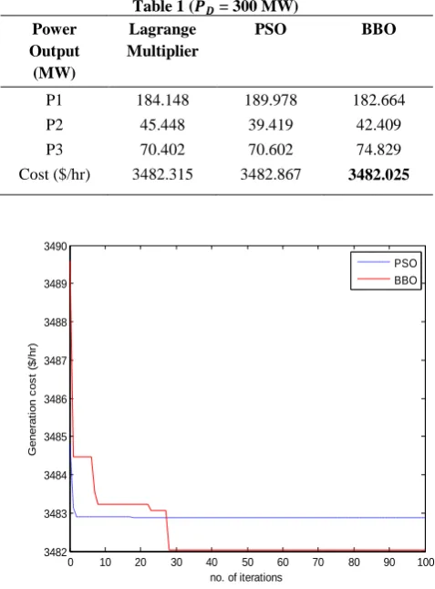
Table 1 shows the total generation cost and power output of each generator obtained by Lagrange multiplier, PSO and BBO methods. Convergence characteristics of PSO and BBO are shown in figure 1.
Table 1 (𝑷𝑫 = 300 MW)
Power Output (MW)
Lagrange Multiplier
PSO BBO
P1 184.148 189.978 182.664
P2 45.448 39.419 42.409
P3 70.402 70.602 74.829
Cost ($/hr) 3482.315 3482.867 3482.025
Figure 1: Convergence characteristics of PSO and BBO (three generator system)
Case 2: Six Generator System
For this system, population size is 30. Maximum number of iterations is taken as 100.
PSO parameters used are [1]:
Minimum inertia weight factor 𝑤𝑚𝑖𝑛 = 0.4
Maximum inertia weight factor 𝑤𝑚𝑎𝑥 = 0.9
Acceleration constants 𝑐1 = 2, 𝑐2 = 2
Table 2 shows the total generation cost and power output of each generator obtained by Lagrange multiplier, PSO and BBO methods. Convergence characteristics of PSO and BBO
are shown in figure 2.
0 10 20 30 40 50 60 70 80 90 100
3482 3483 3484 3485 3486 3487 3488 3489 3490
no. of iterations
G
e
n
e
ra
ti
o
n
c
o
s
t
($
/h
r)
[image:3.595.310.549.151.474.2]Table 2 (𝑷𝑫 = 1263 MW) Power
Output (MW)
Lagrange Multiplier
PSO BBO
P1 446.707 446.706 436.150
P2 171.257 171.258 177.708
P3 264.105 264.105 269.735
P4 125.216 125.214 127.812
P5 172.118 172.118 167.760
P6 83.593 83.593 83.319
Cost ($/hr) 15275.931 15275.930 15270.803
Figure 2: Convergence characteristics of PSO and BBO (six generator system)
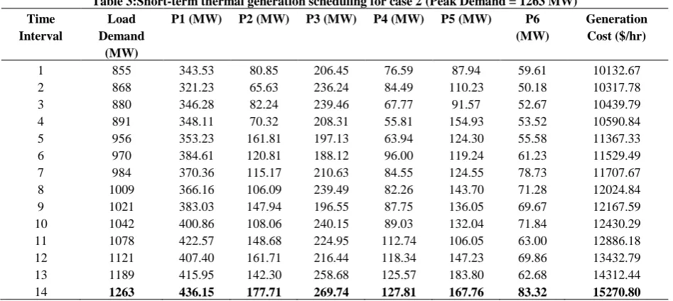
The optimal thermal generation schedule for the six generator system is shown in table 3 for a peak demand of 1263 MW.
6.
CONCLUSION
In this paper, the BBO algorithm has been applied to ED problems. The performance of this algorithm has been compared with the conventional Lagrange multiplier method and the PSO algorithm by employing two different test systems and it has been found that BBO algorithm obtains comparative results with respect to these methods. Results obtained through BBO clearly exhibit an improved solution quality and stable convergence characteristics. Global search capability is enhanced and premature convergence is avoided. Also, a 24-hour short-term thermal generation schedule has Been presented for the six generator system to further add to the effectiveness of the BBO algorithm. Table 2 shows the total generation cost and power output of each generator obtained by Lagrange multiplier, PSO and BBO methods. Convergence characteristics of PSO and BBO are shown in figure 2.
7.
ACKNOWLEDGEMENTS
[image:4.595.47.286.78.461.2]The author would like to thank Dan Simon, Associate Professor in the Electrical and Computer Engineering Department, Cleveland State University, whose paper on BBO has helped a lot to carry out the work presented in this paper.
Table 3:Short-term thermal generation scheduling for case 2 (Peak Demand = 1263 MW) Time
Interval
Load Demand
(MW)
P1 (MW) P2 (MW) P3 (MW) P4 (MW) P5 (MW) P6
(MW)
Generation Cost ($/hr)
1 855 343.53 80.85 206.45 76.59 87.94 59.61 10132.67
2 868 321.23 65.63 236.24 84.49 110.23 50.18 10317.78
3 880 346.28 82.24 239.46 67.77 91.57 52.67 10439.79
4 891 348.11 70.32 208.31 55.81 154.93 53.52 10590.84
5 956 353.23 161.81 197.13 63.94 124.30 55.58 11367.33
6 970 384.61 120.81 188.12 96.00 119.24 61.23 11529.49
7 984 370.36 115.17 210.63 84.55 124.55 78.73 11707.67
8 1009 366.16 106.09 239.49 82.26 143.70 71.28 12024.84
9 1021 383.03 147.94 196.55 87.75 136.05 69.67 12167.59
10 1042 400.86 108.06 240.15 89.03 132.04 71.84 12430.29
11 1078 422.57 148.68 224.95 112.74 106.05 63.00 12886.18
12 1121 407.40 161.71 216.44 118.34 147.23 69.86 13432.79
13 1189 415.95 142.30 258.68 125.57 183.80 62.68 14312.44
14 1263 436.15 177.71 269.74 127.81 167.76 83.32 15270.80
0 10 20 30 40 50 60 70 80 90 100 1.52
1.53 1.54 1.55 1.56 1.57 1.58x 10
4
number of iterations
g
e
n
e
ra
ti
o
n
c
o
s
t
($
/h
r)
[image:4.595.62.536.551.763.2]15 1176 387.03 163.05 263.04 108.09 161.62 93.16 14152.62
16 1219 461.91 138.82 234.93 126.30 176.58 80.45 14712.28
17 1089 374.20 142.04 214.41 105.23 162.76 90.36 13041.52
18 1058 420.89 120.92 196.71 90.87 166.99 61.61 12642.95
19 1010 385.23 116.58 250.73 110.40 83.71 63.34 12046.74
20 986 362.83 100.45 213.85 106.04 140.55 62.28 11738.89
21 945 345.65 141.59 229.73 65.87 78.58 83.56 11253.35
22 910 400.69 105.53 198.86 80.05 74.31 50.54 10794.54
23 887 379.97 100.16 167.30 58.19 111.85 69.50 10526.95
24 855 343.53 80.85 206.45 76.59 87.94 59.61 10132.67
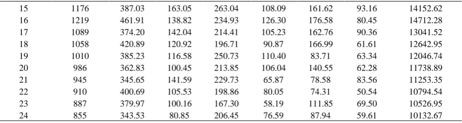
[image:5.595.67.533.71.195.2]Load profile during 24-hour interval for the six generator system is shown in figure 3.
Figure 3: Load profile for 24-hour interval (six generator system)
8. REFERENCES
[1]Kothari, D. P. andDhillon, J. S. 2010. ‘Power System Optimization’, 2nd edition, PHI, New Delhi
[2] Mohamed-Nor, K. and Rashid, A. H. A. 1991. ‘Efficient economic dispatch algorithm for thermal unit commitment’, IEE Proceedings C, vol. 138 (3), pp. 213-217
[3] Chung-Lung, Chen and ChenNanming 2001. ‘Direct search method for solving economic dispatch problem considering transmission capacity constraints’, IEEE Trans. on Power Systems, vol. PWRS-16 (4), pp. 764-769
[4] Brar, Y. S., Dhillon J. S. and Kothari D. P. 2002. ‘Multi-objective load dispatch by fuzzy logic searching weightage pattern’, Electric Power Systems Research, vol. 63 (2), pp. 149-160
[5] Lee, K. Y., Sode-Yome A. and Park J. H. 1998. ‘Adaptive Hopfield neural networks for economic load dispatch’, IEEE Trans. on Power Systems, vol. 13 (2), pp. 519-526
[6] Yalcinoz, T.and Short M. J. 1998. ‘Neural networks approach for solving economic dispatch problem with transmission capacity constraints’, IEEE Trans. on Power Systems, vol. 13, pp. 307-313
IEEE Trans. on Power Systems, vol. 8 (3), pp. 1325-1332
[8] Sheble, G. B. and Brittig K. 1995. ‘Redefined genetic algorithm – economic dispatch example’, IEEE Trans. on Power Systems, vol. 10, pp. 117-124
[9] Fogel, D. B. 2000. ‘Evolutionary computation: Towards a new philosophy of machine intelligence’, 2nd edition, Piscataway, NJ: IEEE Press
[10] Eberhart, R. C. and Shi Y. 1998.‘Comparison between genetic algorithms and particle swarm optimization’, Proceedings of IEEE Int. Conf. on Evol.Comput., pp. 611-616
[11] Gaing, Z. L. 2003. ‘Particle swarm optimization to solve the economic dispatch considering the generator constraints’, IEEE Trans. on Power Systems, vol. 18 (3), pp. 1187-1195
[12] Ratnaweera, A., Halgamuge S. K. and Watson H. C. 2004.‘Self-organizing hierarchical particle swarm optimizer with time varying acceleration coefficients, IEEE Trans. on Evol.Comput., vol. 8 (3), pp. 240-255
[13] Selvakumar, A. I. and Thanushkodi K. 2007. ‘A new particle swarm optimization solution to nonconvexeconomic dispatch problems, IEEE Trans. on Power Systems, vol. 22 (1), pp. 42-51
0
200
400
600
800
1000
1200
1400
1
2
3
4
5
6
7
8
9 10 11 12 13 14 15 16 17 18 19 20 21 22 23 24
L
o
ad
(M
W
)
[14] Panigrahi, B. K. and Pandi V. R. 2008 ‘Bacterial foraging optimization: Nelder-Mead algorithm for economic load dispatch’, Generation, Transmission and Distribution, IET, vol. 2 (4), pp. 556-565
[15]NomanNasimul, and Iba Hitoshi 2008. ‘Differential evolution for economic load dispatch problems’, Electric Power Systems Research, vol. 78, pp. 1322-1331
[16]Mezura-Montes, E., Velazquez-Reyes, J. and Coello C. A. C. 2006. ‘Modified differential evolution for constrained optimization’, Proceedings of the 2006 IEEE Congress on Evolutionary Computation, pp. 332– 339
[17]Simon D. 2008.‘Biogeography-based optimization’, IEEE Trans. on Evol.Comput., vol. 12 (6), pp. 702-713
[18] Bhattacharya A. and Chattopadhyay P. K. 2010. ‘Biogeography-based optimization for different
economic load dispatch problems’, IEEE Trans. on Power Systems, vol. 25(2), pp. 1064-1077
[19]Roy, P. K., Ghoshal S. P. and Thakur S. S. 2009 ‘Biogeography based optimization technique applied to multi-constraints economic load dispatch problems’, IEEE T & D Asia
[20]Kothari, D. P. and Parmar K. P. Singh 2006. ‘A novel approach for eco-friendly and economic power dispatch using MATLAB’, International Conference on Power Electronics, Drives and Energy Systems, PEDES ’06, pp. 1-6