GUIDING FEATURE BASED SAR IMAGE ALIGNMENT USING BAG OF WORDS MODEL

FIBROUS ROOT MODEL

IN BATIK PATTERN GENERATION

PURBA DARU KUSUMA

School of Electrical Engineering, Telkom University, Bandung, Indonesia

E-mail: [email protected]

ABSTRACT

Batik is one of famous cultural heritage in Indonesia. One effort to preserve batik is by exploring new patterns. One of popular pattern is floral pattern. In this research, fibrous root model is proposed and is combined with the traditional batik pattern. This model is developed by combining root growth model based on L-system and random walk. In this research, the fibrous root model has been implemented into computer based batik pattern generation with some alternatives: single direction, random direction, and radial direction. Based on the test, split ratio has positive correlation with the average number of segments. Die ratio has negative correlation with the number of segments. The maximum deviation angle makes the root growth wider. The number of seeds and the number of iterations have positive correlation with the number of segments. The increasing of the number of seeds makes the complexity grows linearly. The increasing of the number of iterations makes the complexity grows logarithmically.

Keywords: Fibrous Root, Batik, Pattern Generation, L-System, Stochastic

1. INTRODUCTION

Batik is one of cultural heritage in Indonesia. There are various patterns that can be found in Indonesia. It is because there are many tribes in Indonesia and their cultures are very diverse. Batik has been also recognized as world cultural heritage by UNESCO. As cultural heritage, many efforts have been done to preserve batik from its extinction. Even there are many traditional classic patterns, exploring new patterns is important too. In traditional way, the pattern is developed manually. In the other hand, computational technology can improve this process [1-3]. One of the popular method is fractal technology [1][2]. By computational technology, new pattern design can be generated faster and more various.

One popular pattern in decorative pattern is the floral pattern. Floral pattern can be found easily in East Java batik, such as Madura or Banyuwangi batik. Floral pattern is also can be found in other country traditional pattern such as Persian pattern [4]. Most popular floral pattern is flower pattern. The next popular patterns are leaf and climbing plant patterns. This research is motivated by the fact that root pattern is very rare and is difficult to be found in batik pattern design. So, developing root growth pattern as beautiful batik pattern is challenging.

The objective of this research is to develop fibrous root pattern in batik pattern generation by combining L-system and random walk. This research proposes realistic and simple root growth model. Then, this model is implemented to generate batik pattern. This model must be realistic so people still recognize that the pattern is root pattern. This model must be simple so the computation still light because this basic root pattern will be added into batik pattern generation application. In this research, the type of the root that is modeled is fibrous root.

This model is divided into two works. The first work is generating set of nodes that represents root growth pattern. The second work is generating batik object at the specified nodes. The root pattern is developed by combining modified L-system and random walk. L-system is used as the deterministic part. Random walk is used as the stochastic part. This model implements random walk with drift.

2. LINDENMAYER SYSTEM (L-SYSTEM)

There are many techniques in modeling plant growth. One of them is L-system that was introduced by Lindenmayer. This method varies from simple to complex form [5]. This method has been used to model root [6], branch, leaf, and flower. This method also has been improved and combined with other method [7-11]. L-system was also used to develop plant like model [12-16]. The other method is random walk. The other method is random walk that was used with the assumption that plant growth is stochastic and the plant behavior cannot be predicted exactly even many parameters have been used [17-20]. Other method used complex biological mechanism such as elongation, mortality, and gravity [21].

One popular method in modeling plant growth is Lindenmayer or L-system. Basically, this method uses rewriting concept. The mechanism of rewriting method is replacing part of initial simple object using rewriting rules. Basically, this method is deterministic. The example of simple L-system is the algorithm in Figure 1.

Figure 1: Simple L-System Algorithm

Figure 2: Visualization Example of Simple L-System

In Figure 1, there are two types of node, branch and flower. The initial node is branch. If the node is a branch, then new branch and new flower a created. If the node is flower, then there is not any action is done. Variable n represents the number of iterations. Variable m represents the number of nodes. The status of node is life or die. The result of this algorithm can be seen in Figure 2.

Based on this simple method, L-system then was used, modified, and combined with other method to model more specific plant growth. Suhartono combined L-system and Fuzzy Mamdani to model Zinnia Elegans growth [7]. Castellanos used L-system to model plant death process simulation [8]. Meng used L-system to model to model wheat rooting [10]. Hamon used L-system to model 3D virtual plant simulation [11].

L-system was also used to model plant like object. Davoodi used L-system to model human bronchial tree [12]. De Campos combined L-system with genetic algorithm to develop artificial neural structure and used it to simulate the effect of a new drug on breast cancer [14]. Liu used L-system to model blood vessels in surgery simulator [16].

3. FIBROUS ROOT

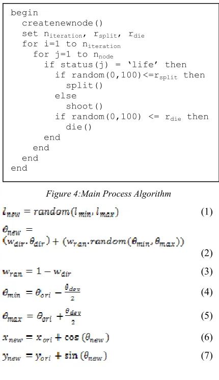
Fibrous root is root type that is found in monocotyledonous plant, such as corn, wheat, palm, banana, and orchid [22]. It is formed by thin, many, and moderately branching roots growing from the stem. The opposite of the fibrous root is tap root. Tap root system is usually found in dicotyledonous plant, such as mango tree, in tap root system, there are one central and the largest root. The other roots spread laterally from this main root. The form of fibrous root is illustrated in Figure 3 [23].

Figure 3: Fibrous Root Illustration begin

node[0] ← branch status[0] ← life for i=1 to n

m ← length(node) - 1 for j=0 to m

if node[j] = branch and status[j] = life then node[m] ← flower node[m+1] ← branch status[j] ← die end

4. PROPOSED MODEL

The proposed model is divided into two steps. The first step is generating root model as a set of nodes. The second step is placing batik objects at the selected nodes. In the first step, the root model is generated by the combination of simplified L-system and random walk method. The output of the first step is a set of nodes with their coordinate that describes the fibrous root form and the status of the node because each status of nodes will be presented with certain batik object. In the second step, the set of nodes will be filled with specific nodes, lines, and or curves that form specific batik objects. The output of the second step is the batik image that visualizes fibrous root.

Several autonomous agents are generated to draw fibrous root during the first step. Each agent represents a stem or a seed. The stem position is the initial position of the root growth. Each agent acts independently and doesn’t interact with other agents. The root growth process run in iterative process and will be terminated after the iteration stops.

There are three activities that are used in this root growth process. Shoot is the activity that the branch extends the length with specific additional length and angle. Split is the activity that the branch is split into two branches. Each branch has its own length and angle. Die is the activity that terminates the growth of the branch. If the status of a branch is dies, this branch will not grow anymore.

The action that is chosen by the agent is probabilistic. There are two ratios that are used, the split ratio (rsplit) and die ratio (rdie). Split ratio is the

ratio that determines the branch will split. Die ratio is the ratio that determines the branch will die. The main algorithm of this process is described in Figure 4. In this main process algorithm, shoot function means system will create one new node and split function means system will create two new nodes. The new node status is set as life. Die function changes the status of the selected node into die.

Creating new branch means creating new node with specific coordinate and angle (xnew, ynew,

θnew). This coordinate is determined by position and

the angle of the origin node (xori, yori, θori), the

maximum angle deviation θdev, and the length of

new branch (lnew). The coordinate and angle of the

new node is determined by Equation 1 to 7. The lnew

is determined randomly between minimum length

(lmin) to maximum length (lmax). θdir is the

deterministic direction of root growth that is set manually. Variable wdir is the weight that

determines that the root direction follows deterministic part. Variable wran is the weight that

determines that the root direction follows random part.

Figure 4:Main Process Algorithm

(1)

(2)

(3)

(4)

(5)

(6)

(7)

5. IMPLEMENTATION

This model has been implemented to create fibrous root pattern batik image. The implementation is developed by using PHP language. The result is JPEG formatted image. The image size is 1000 x 1000 pixels. There are four types of image. The difference is in the starting point position and the deterministic direction of the root growth. In the first type, the starting point position is placed on the top position and placed horizontally with same distance and the roots grow in same deterministic direction. In the second type, the starting point position is determined randomly and the roots grow in the same direction. In the

begin

createnewnode()

set niteration, rsplit, rdie

for i=1 to niteration

for j=1 to nnode

if status(j) = ‘life’ then

if random(0,100)<=rsplit then

split() else shoot()

if random(0,100) <= rdie then

third type, the starting point position is placed randomly and the deterministic direction is set randomly too. In the fourth type, there are groups of roots. The deterministic direction is radial.

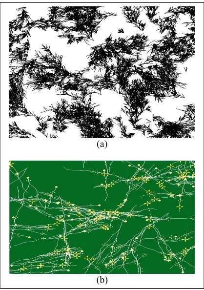
The first type is fibrous root pattern batik image with the starting point position is at the top of the image and the root grows in the same deterministic direction. There are some stems that are used in this image. The stems are placed at the top of the image. The stems are arranged horizontally. Every stem has same distance with its neighbor. The visualization of the first type is illustrated in Figure 5. Figure 5a illustrates the root growth pattern. Figure 5b illustrates the finalized batik image.

Figure 5: Single Direction Type Fibrous Root

Figure 6: Single Direction Type Fibrous Root with Randomized Starting Position

In the second type, the starting point position of stem is determined randomly and the roots grow with the same deterministic direction. The visualization of this type is illustrated in Figure 6. Figure 6a illustrates the root growth pattern. Figure 6b illustrates the finalized batik image.

In the third type, the starting point position of the stem and the deterministic direction are determined randomly. The visualization of this type is illustrated in Figure 7. Figure 7a illustrates the root growth pattern. Figure 7b illustrates the finalized batik image.

Figure 7: Random Direction Type Fibrous Root

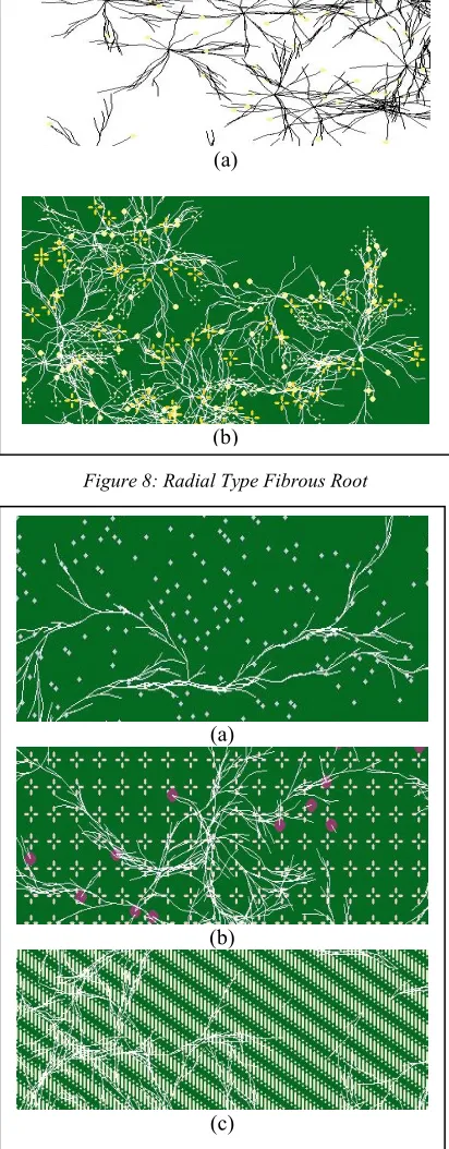
The concept of the fourth type is creating the radial root growth pattern. To create it, the roots are collected into groups. There are some specific numbers of stems in each group. In a group, the position of stems is same. The position of stem groups is determined randomly. To make radial growth, the deterministic direction of each stem in one group has fixed angle gap with its neighbor. For example, if the group consists of four stems, the direction of the stems is 0, 90, 180, and 270 degree consecutively. If the group consists of six stems, the direction of the stems is 0, 60, 120, 180, 240, and 300 degree consecutively. The visualization of this type is illustrated in Figure 8. Figure 8a

(a)

(b)

(a)

(b) (a)

illustrates the root growth pattern. Figure 8b illustrates the finalized batik image.

Figure 8: Radial Type Fibrous Root

Figure 9: Improvisation Basic Fibrous Root with Existing Batik Pattern

This basic model can be implemented with some improvisations. The first final pattern is developed by adding dot in every origin seed and flower pattern in every die segment as seen in Figure 5b, Figure 6b, Figure 7b, and Figure 8b. The other modification can be added in the background. In Figure 9a, randomized dots are added as image background. In Figure 9b, Kawung pattern is added as image background. In Figure 9c, Parang pattern is added as image background.

6. DISCUSSION

Based on the proposed model and the image result that has been generated by using the model, the generated root met the fibrous root characteristic which is different with tap root [22]. However, there are differences between the existing model and the proposed model. In the existing model, the root segment length is determistic [6]. In the other hand, in this research, the root segment length is stochasticly distributed. In the existing model, the soil model is used in the calculation [6]. In this research, the soil content is ignored to reduce the complexity. The existing model used continuous approach [21]. In the other hand, this research uses discrete approach.

Based on the visual appearance of the result image, the model can generate general fibrous root. It can be seen by comparing fibrous root image in Figure 3 and Figure 5a. The root that is generated by the model has fibrous root characteristic. The root does not contain main root. There are root segments that split and create new root segment. The root length is various. It means that there is stochastic aspect in root growth model. However, the root growth is not fully stochastic. Based on Figure 3, it can be seen that the root tends to avoid sun light. This requirement has been accomodated in Equation 2 which combines deterministic aspect and stochastic aspect in certain weight.

In some plants, such as orchid, a seed initiates many root segments. After being initiated, the root segment tends not to split. The root just extends its length. The splitting behavior is very rare. This behavior is illustrated in Figure 10. This root behavior has been accomodated in this proposed model. This behavior is similar to result image in Figure 8a. The occurrence of the splitting behavior can be reduced by setting the split ratio value low.

(a)

(b)

(c) (a)

Figure 10: Root with Many Initiated Segments and Rare Splitting Bahavior

However, there is limitation in this model so there is root behavior that has not been accomodated in this model. In the real world, the root follows the medium. For example, when the root segment hits the pot, the root cannot cross the pot and it follows the pot. The root then follows the pot surface. The proposed model has not accomodated this behavior yet. In this model, if the root hits the pot, the root still grows crossing the pot. This behavior can be seen in Figure 11.

Figure 11: Root Behavior That Follows The Surface Medium

In this research, there are two test groups. The first group is analyzing the relation between input parameters and the output. The second group is analyzing the algorithm complexity. The input parameters that have been evaluated are split ratio

(rsplit), die ratio (rdie), maximum deviation angle

(θdev), and directed weight (wdir). The algorithm complexity test has been done by using Big O analyzes.

There are some limitations in this research testing. The maximum split ratio is 50. The maximum die ratio is 80. The maximum deviation

angle is 180 degrees. The maximum number of seeds is 90 seeds. The maximum number of iterations is 90 iterations. These limitations, especially in split ratio, number of seeds and number of iterations, are based on the computation complexity that burdens the calculation.

The first test is evaluating the split ratio value (rsplit) as input parameter with number of root segments (ns) as output parameters. Logically, if the

rdie is zero and rsplit is zero, the value of ns is same with the number of iteration (ni). it is because the root will never die and there is not any splitting activities. In this test, the value of rdie is set zero. The value of ni is 10. The number of seeds is 500. The output is the average ns for 500 seeds after ten

iterations. The result is described in Table 1. Based on the data in Table 1 and the data trend in Figure 12, it can be seen that when the split ratio grows linearly, the average number of segments grows exponentially. Because the average number of segments can be used as complexity evaluation, the increasing of split ratio makes the complexity in computation higher and the trend is exponential.

Table 1: Relation between Split Ratio and Average Number of Segments

Split Ratio (rsplit)

Average Number of Segment (ns)

0 10

5 13.2

10 18.1

15 25.3

20 39.7

25 65.8

30 114.5

35 173.6

40 354.3

45 730.4

50 973.9

The second test is evaluating the die ratio value (rdie) as input parameter with number of root segments (ns) as output parameter. It is same with the assumption in the first test. Logically, if the rdie is zero and rsplit is zero, the value of ns is same with the number of iteration (ni). This is because the root will never die and there is not any splitting activity. In this test, the value of rsplit is set zero. The value of

ni is 10. The number of seeds is 500. The output is the average ns for 500 seeds after ten iterations. The

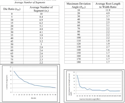
result is described in Table 2. Based on the data in Table 2 and data trend in Figure 13, it can be seen that when the split ratio grows linearly, the average number of segments grows negative exponentially. As in split ratio, by using the trend of the average number of segments, the increasing of die ratio makes the computation complexity lower with the trend is negative exponential. So, the die ratio can be the balancing counterpart to the split ratio.

Table 2: Relation between Die Ratio and Average Number of Segments

Die Ratio (rdie)

Average Number of Segment (ns)

0 10

5 8.4

10 6.9

15 6.2

20 5.1

25 4.8

30 4.1

35 3.8

40 3.3

45 3.2

50 3

55 2.8

60 2.6

65 2.6

70 2.5

75 2.3

80 2.2

Figure 13: The Trend of Relation between Die Ratio and the Average Number of Segments

The third test is evaluating the effect of maximum deviation angle (θdev) to the ratio between length and width of the root. In this test, the die ratio is set 50 and the split ratio is set 50. The input parameter is θdev. The output parameter is the ratio between the length of the root and the width of the root. It is assumed that bigger value of θdev creates lower value of this ratio. The directed weight is set 0. The number of seeds is 500. The number of iteration is 50. The result is described in Table 3 and Figure 14. Based on data in Table 3, it is proven that lower maximum deviation angle creates lower length to width ratio of the root. Based on trend in Figure 14, it can be seen that when the maximum deviation angle grows linearly, the length to width ratio of the root grows negative exponentially.

Table 3: Relation between Maximum Deviation Angle and Average Number of Length and Width Ratio of the

Root

Maximum Deviation Angle (θdev)

Average Root Length to Width Ratio

10 11.9

20 4.9

30 3.7

40 3.8

50 2.5

60 3.1

70 2.2

80 2.2

90 2.2

100 2.2

110 1.8

120 1.9

130 2.7

140 1.6

150 1.7

160 1.6

170 1.7

180 1.7

The next testing group is complexity testing. The complexity testing is done by evaluating the calculation load when the data size is increasing. In this research, there are two data size that have been evaluated. They are the number of seed and the number of iteration.

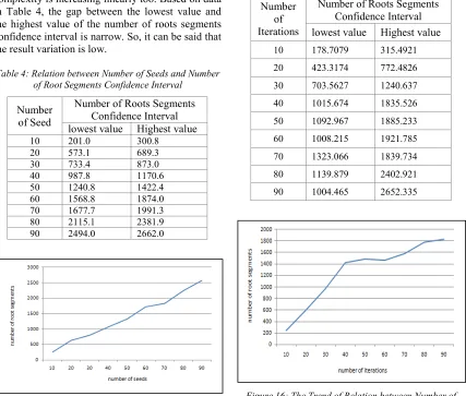
The first test is calculating the number of root segment if the number of seed increases. In this test, the number of seed grows from 10 to 90 with the interval is 10. The number of iteration is 10. There are ten simulation sessions for every number of seed value. The confidence level is 90 percents. The confidence interval result can be seen in Table 4 and the trend result can be seen Figure 15. Based on trend data in Figure 15, it can be seen that when the data size is increasing linearly, the complexity is increasing linearly too. Based on data in Table 4, the gap between the lowest value and the highest value of the number of roots segments confidence interval is narrow. So, it can be said that the result variation is low.

Table 4: Relation between Number of Seeds and Number of Root Segments Confidence Interval

Number of Seed

Number of Roots Segments Confidence Interval lowest value Highest value 10 201.0 300.8

20 573.1 689.3 30 733.4 873.0 40 987.8 1170.6 50 1240.8 1422.4 60 1568.8 1874.0 70 1677.7 1991.3 80 2115.1 2381.9 90 2494.0 2662.0

Figure 15: The Trend of Relation between Number of Seeds and Number of Root Segments

The second test is calculating the number of root segments if the number of iteration increases. In this test, the number of iteration grows

from 10 to 90 with the number of interval is 10. There are ten simulation sessions for every number of iterations. The confidence level is 90 percents. The confidence interval result can be seen in Table 5 and the trend result can be seen in Figure 16. Based on data in Figure 16, it can be seen that when the data size is growing linearly, the complexity grows logarithmically. Based on the data in Table 5, it can be seen that the variation of the number of roots segments variation is very wide. It is because some roots have stopped growing while others still grow during the iterations. So, the increasing the number of iterations makes the variation wider.

Table 5: Relation between Number of Iterations and Number of Root Segments Confidence Interval

Number of Iterations

Number of Roots Segments Confidence Interval lowest value Highest value

10 178.7079 315.4921

20 423.3174 772.4826

30 703.5627 1240.637

40 1015.674 1835.526

50 1092.967 1885.233

60 1008.215 1921.785

70 1323.066 1839.734

80 1139.879 2402.921

90 1004.465 2652.335

7. CONCLUSION AND FUTURE WORK

Based on the explanation above, this research has met its purpose, which is generating batik pattern based on fibrous root model. This is also the novelty of this research. As an art design, in this research, the basic root growth has been manipulated. In this research, there are three types of root growth direction, which are: uniform direction, random direction, and radial direction. This root model has been modified with other batik patterns too. In this research, the complexity testing also has been done and makes some results. The increasing of split ratio makes the complexity grows exponentially. The increasing of die ratio makes the complexity grows negative exponentially. So, the die ratio acts as balancing counterpart to the split ratio. The increasing of maximum deviation angle makes the root length to width ratio grows negative exponentially. The increasing of the number of seeds makes the complexity grows linearly. The increasing of the number of iterations makes the complexity grows logarithmically.

There are many opportunities in computer aided batik pattern generation. In floral pattern, many plants with their own characteristic can be used as basic model to create batik pattern. The future research direction is in developing batik pattern based on the specific parts of the plant or the entire of the plant.

REFERENCES:

[1] Y. Li, C. J. Hu, and X. Yao, “Innovative Batik Design with an Interactive Evolutionary Art System”, Journal of Computer Science and Technology, vol. 24(6), 2009, pp. 1035-1047. [2] R. Yulianto, M. Hariadi, M. H. Purnomo, and

K. Kondo, “Iterative Function System Algorithm Based a Conformal Fractal Transformation for Batik Motive Design”,

Journal of Theoretical and Applied

Information Technology, vol. 62(1), 2014, pp. 275-280.

[3] S. Liu, J. Wang, “Computer Technology Imitate Traditional Dyeing Patterns”,

Proceeding of Technical Congress on

Resources, Environment, and Engineering, Hongkong, September 2014, pp. 277-282. [4] K. Etemad, F. F. Samavati, and P.

Prusinkiewicz, “Animating Persian Floral Patterns”, Proceeding of Computational

Aesthetics in Graphics, Visualization, and Imaging, Lisbon, June 2008.

[5] P. Prusinkiewicz, A. Lindenmayer, The Algorithmic Beauty of Plants, Springer-Verlag: New York, 1990.

[6] D. Leitner, A. Schneff, “Root growth Simulation Using L-Systems”, Proceeding of Algorithmy, Podbanske, March 2009, pp. 313-320.

[7] Suhartono, M. Hariadi, and M.H. Purnomo, “Plant Growth Modeling of Zinnia Elegans Jacq Using Fuzzy Mamdani and L-System Approach with Mathematica”, Journal of

Theoretical and Applied Information

Technology, vol. 50(1), 2013, pp. 1-6.

[8] E. Castellanos, F. Ramos, and M. Ramos, “Semantic Death in Plant’s Simulation Using Lindenmayer Systems”, Proceeding of 10th

International Conference on Natural

Computation (ICNC), Xiamen, August 2014, pp. 360-365.

[9] S. Hanafin, S. Datta, and B. Rolfe, “Tree Facades: Generative Modelling with an Axial Branch Rewriting System”, Proceeding of 16th International Conference on Computer-Aided

Architectural Design Research in Asia

(CAADRIA), New South Wales, April 2011, pp. 175-184.

[10]J. Meng, X. Y. Guo, S. L. Lu, B. X. Xiao, and W. L. Wen, “Modeling Rooting in Wheat Using Lindenmayer System”, Proceeding of 4th

International Conference on Intelligent

Computation Technology, Guangdong, March 2011, pp. 121-124.

[11]L. Hamon, E. Richard, P. Richard, and J.L. Ferrier, “Real-time Interactive L-system: A Virtual Plant and Fractal Generator”,

Proceeding of 5th International Conference on Computer Graphics Theory and Applications, France, May 2010, pp. 370-377.

[12]A. Davoodi, R.B. Boozarjomehry, “Developmental Model of an Automatic Production of the Human Bronchial Tree Based on L-system”, Computer Methods and Programs in Biomedicine, vol. 132, 2016, pp. 1-10.

[13]D. Bie, J. Zhao, X. Wang, and Y. Zhu, “A Distributed Self Reconfiguration Method Combining Cellular Automata and L-systems”,

IEEE International Conference on Robotics and Biomimetics, Zuhai, December 2015, pp. 60-65.

Networks Through L-system and Evolutionary Computation”, Proceeding of International

Joint Conference on Neural Networks

(IJCNN), Killarney, July 2015.

[15]S. Badura, “Analysis for Effective Approaches Towards Generating of Artificial Neuron Structures”, Proceeding of IEEE International

Symposium on Signal Processing and

Information Technology, Bilbao, December 2011, pp. 130-133.

[16]X. Liu, H. Liu, A. Hao, Q. Zhao, “Simulation of Blood Vessels for Surgery Simulators”,

Proceeding of International Conference on

Machine Vision and Human-Machine

Interface, Kaifeng, April 2010, pp. 377-380. [17]A. Johnsson, C. Karlsson, T. H. Iversen, D. K.

Chapman, and J. Braseth, “Plant Growth and Random Walk – An Experiment for IML-2”,

Proceeding of 5th European Symposium on Life

Sciences Research in Space, Arcachon,

September 1993, pp. 121-125.

[18]A. Klopper, “Random Walks: Root Manoeuvre”, Nature Physics, vol. 11(891), 2015.

[19]M. L. Cain, “Models of Clonal Growth in Solidago Altissima”, Journal of Ecology, vol. 78, 1990, pp. 27-46.

[20]B. Benes, E. U. Millan, “Virtual Climbing Plants Competing for Space”, Proceeding of the IEEE Computer Animation, 2002.

[21]L. Dupuy, P. J. Gregory, and A. G. Bengough, “Root Growth Models: Towards a New Generation of Continuous Approaches”,

Journal of Experimental Botany, vol. 61(8), 2010, pp. 2131-2143.

[22]K. Ajithadoss, Biology: Botany, 1st ed, Tamil Nadu Textbook Corporation, Chennai, 2005. [23] , Roots as Anchors, National Gardening

Association,