LOW COMPLEXITY HEVC INTRA MODE DECISION USING MODES REDUCTION

514

EXTENDED BLOCK NEIGHBOR DISCOVERY PROTOCOL

FOR HETEROGENEOUS WIRELESS SENSOR NETWORK

APPLICATIONS

1_{WOOSIK LEE,} 2*_{NAMGI KIM,} 3_{TEUK SEOB SONG,} 4_{JONG-HOON YOUN}

1, 2_{Department of Computer Science, Kyonggi University, Suwon 16277}

3_{Division of Convergence Computer, Mokwon University, Daejeon 35349}

4_{College of Information Science and Technology, University of Nebraska Omaha, NE 68182}

E-mail: 1_{[email protected],} 2_{[email protected],} 3_{[email protected],} 4_{[email protected]} *_{Corresponding Author: Namgi Kim ([email protected])}

ABSTRACT

For heterogeneous wireless sensor network applications, sensor nodes need diverse duty cycles and energy efficient neighbor discovery protocols (NDPs) so that they can rapidly find their neighbor nodes. However, existing block NDPs have very limited duty cycle sets. To solve this problem, we propose extended block NDP (EBNDP), a protocol that can support diverse duty cycles. EBNDP adaptively generates block candidates depending on duty cycle requirements. It selects block sets based on a heuristic search approach and combines the selected block sets to make a new block design. This combined block design supports the duty cycle requirements and has proper performance that is close to optimal block design regarding latency and energy consumption. To evaluate the effectiveness of EBNDP, we implemented various block combinations depending on the duty cycles and compared the performance of each block combination. We also compared EBNDP with other NDPs such as Quorum, Optimal, Random, and OR-based NDPs. Through experimentation, we showed that EBNDP outperformed other NDPs in all duty cycles.

Keywords: Wireless Sensor Network, Neighbor Discovery Protocol, Block Design

1. INTRODUCTION

This guide provides details to assist authors in preparing a paper for publication in JATIT so that there is a consistency among papers. These instructions give guidance on layout, style, illustrations and references and serve as a model for authors to emulate. Please follow these specifications closely as papers which do not meet the standards laid down, will not be published.

There are many different applications of heterogeneous wireless sensor networks (HWSNs) such as environmental monitoring, tracking systems, and indoor or outdoor location systems. These applications require sensor nodes with diverse duty cycles of different total length and active slots within one cycle [1]. Then, supporting various duty cycles is critical in HWSNs. A duty cycle is the ratio of one period in which a signal is active. Block design-based neighbor discovery protocol (BNDP) is a representative technique to

create sensor node schedules with duty cycles suitable for HWSN applications.

BNDP turns a sensor node’s radio on or off depending on its duty cycle requirements. Each block of sensor scheduling is set to either ‘1’ or ‘0’. If the block number is ‘1’, the sensor nodes turn their radios on to send or receive data packets between sensor nodes. If the block number is ‘0’, the sensor nodes turn their radios off to go into sleep mode to save energy. BNDP uses a balanced incomplete block design (BIBD) which ensures that the sensor nodes have at least one common active slot per cycle. This is known as optimal NDP for symmetric neighbor discovery systems [2].

515 LDC, sensor nodes rarely turn their radio on to exchange data packets, leading to reduced consumption of battery resources and longer lifetime. In HDC, sensor nodes frequently turn their radio on to send and receive data packets. Thus, they rapidly consume their small batteries and have a short lifetime. To design a practical HWSN application, we must consider LDC and HDC simultaneously. However, BIBD cannot support various LDC and HDC as required by HWSN applications.

In this paper, we present a block mixing approach to support diverse duty cycles and compare proposed NDP with the original BNDP in HWSNs. We also address the fundamental questions related to various duty cycles:

1) How can we extend the original BIBD for various duty cycles?

2) Given a block construction schedule for NDP, what is the minimum schedule length and wake-up time of sensor nodes in terms of the number of block construction and block combination direction?

3) What is the best NDP through experimental results in HWSNs?

To answer above questions, we first introduce original BIBD for sensor scheduling. After that, we propose a new neighbor discovery protocol called extended block neighbor discovery protocol (EBNDP) that can support diverse duty cycles and has an excellent performance that is close to the optimal block design. Then, we analyze EBNDP according to the number of block combination and the block combination direction.

To verify the effectiveness of our proposed protocol, we implement a sensor network simulator using CSMA/CA in TinyOS. Through simulation studies, we show that EBNDP guarantees that any two sensor nodes can detect each other within finite time without time synchronization. Moreover, EBNDP can achieve shorter latency compared with other NDPs.

The rest of this paper is organized as follows. Section 2 discusses related work. In Section 3, we discuss block design for neighbor discovery protocols. In Section 4, we introduce a new extended block design-based neighbor discovery protocol called EBNDP and analyze it in Section 5. Section 6 presents our simulation results. Finally, we conclude our paper with a discussion of future research.

2. RELATED WORK

Neighbor Discovery Protocols (NDPs) have been studied for a long time. The goal of NDPs is to reduce energy consumption and latency when initially setting up an HWSN. The ultimate goal is to scan rapidly the neighbor nodes of a sink node, which exchanges data with a gateway node [1]. Block design can be used for NDPs in HWSNs, and it is employed by many research approaches [2, 3, 4, 5, 6, 7] such as BIBD, Quorum, OR-based NDP, and SLEEP. Zheng et al. [2] proposed an ideal block design called BIBD for HWSNs, which guarantees that the sensor nodes have at least one common active slot within one cycle. BIBD proved to be an optimal solution for NDP [2, 8]. However, it cannot support various duty cycles because it has only a limited block set for sensor schedules.

OR-based NDP [3] also uses the BIBD concept for sensor scheduling. OR-based NDP is a new scheme using OR operations by efficiently combining blocks of BIBD. For example, if one sensor node uses block set with length 21, and another sensor node has length 7 block set, OR operations combine two different block sets of 7 and 21 block set. After operations, new block set is two properties of 7 and 21 block set. If one of sensor nodes uses created block set, which has two properties of 7 and 21 block set, for their scheduling, they must have common active slots with other sensor nodes with scheduling of 7 and 21 block sets. However, OR-based NDP is not good way in terms of energy consumption, because new block set has lots of active slots.

XOR-based NDP [13] is similar to OR-based NDP, but XOR-based NDP uses XOR operation rather than OR operator. Moreover, XOR-based NDP has similar block combination process to combine block sets for sensor scheduling. However, Xbased NDP has lower active slots than OR-based NDP. That is, in terms of energy consumption, Xbased NDP is better than OR-based NDP. However, OR-OR-based and XOR-OR-based NDPs did not solve the problem of BIBD which is providing diverse duty cycles for HWSN applications.

516 for low-duty cycle, sensor nodes wake frequently up to find their neighbors. That is, Quorum-based NDP is not good method in terms of energy consumption

SLEEP [7] uses a sleep scheduling vector of length n to generate a new block scheduling. Its scheduling blocks are constructed from an algebraic structure with a finite number of elements called a Galois field (GF). SLEEP can make various duty cycles for sensor schedules. Moreover, its performance is better than that of Quorum-based NDP. However, SLEEP needs additional tag values like a sensor’s identification number and global positioning system for time synchronization.

3. BLOCK DESIGN FOR NEIGHBOR DISCOVERY PROTOCOL

Block design can be used for NDPs because the inside of each block has consecutive ‘1’ or ‘0’ digits. The presence of ‘1’ indicates that the sensor nodes’ radio is on, and a ‘0’ indicates that the radio is off. ‘1’ represents an active slot where a sensor turns on its radio module and ‘0’ denotes a sleep slot where a sensor turns off its radio module. Figure 1 shows a partial block design. If sensor nodes use this block design for their scheduling, they first, second, forth, and seventh turn a radio on, and third, fifth, and sixth, turn it off.

Figure 1: Neighbor Discovery Protocol using Block Design

Then, we calculate the number of total slots T(x),

active slots AT(x), and sleep slots ST(x) if a sensor

node x uses its schedule to where is a

permutation of a node x with active and sleep slots.

For example, if sensor node uses 1,1,0,1,0,0,1 for the neighbor discovery protocol,

then 7, 4, and 3. We

also know its duty cycle, which is

100% 100% 57.1% using a duty cycle equation.

4. EXTENDED BLOCK NEIGHBOR DISCOVERY

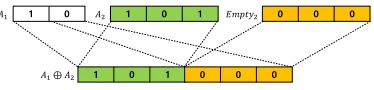
In this section, we introduce a new extended block design-based neighbor discovery protocol called EBNDP. EBNDP combines two different

block designs into one new block design. We use ⊕ as block combination operator. For example, let node 1 have 1,0 and node 2 have

1,0,1 , then, all ‘1’s of are changed by 1,0,1 , and all ’0’s are changed by

0,0,0 with the same size as . After that, EBNDP

defines a new block set ⨁

1,0,1,0,0,0 .

Figure 2: Extended block neighbor discovery schedules using block combination calculation

Then, we can also define a duty cycle for the combination block of node 1 and node 2 as follows:

, 100

(1)

5. ANALYSIS OF EXTENDED BLOCK NEIGHBOR DISCOVERY PROTOCOL

In this section, we analyze EBNDP under two different views. First, we build new block designs using EBNDP to take block combinations from 2 to 5 blocks. Second, we show the relationship between block forward combination and backward combination at block combination time. These use the EBNDP construction method for combining block designs.

5.1 The number of Block Combination

In this section, we show different block designs using EBNDP at the same duty cycle. We denote the number of block construction by , where n is

the number of combinations of block designs. For example, means that a new block design is generated from three different block designs

, , based on EBNDP, where

, , , , . Table 1

shows various block combinations at near 1% duty cycle from 2 to 5 block combinations.

1 1 0 1 0 0 1

On On Off On Off Off On

1 0 1 0 1

1 0 1

0 0 0

0 0 0

517 Table 1: Block Combinations With Near 1% Duty Cycle

Block Combination

C2=57x57 ⊕ 183x183 10431 1.07%

C3= 13x13 ⊕ 183x183

⊕ 7x7 16653 1.00%

C4= 13x13 ⊕ 31x31

⊕ 7x7 ⊕ 7x7 19747 1.09%

C5= 7x7⊕13x13

⊕7x7⊕7x7 ⊕7x7 31213 1.03%

As shown in Table 1, all the block combinations have near 1% duty cycle, but they have different total lengths. Especially, a high block combination like C5 has a longer length than a low block combination like C2. In a real neighbor discovery environment, this is very important because a cycle’s total length is the waiting time to find neighbor nodes after packet drop or at initial setup.

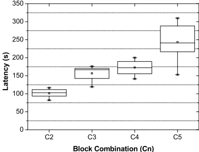
Figure 3: Energy Consumption each block combination with same duty cycle and different block construction

Figure 3 and Figure 4 show average energy consumption and latency depending on four different block designs. In these graphs, outperforms others regarding latency and energy consumption. Moreover, the standard deviation of is lower than that of others. Based on these results, we consider block combinations generated from two block designs.

5.2 Block Combination Direction

This section focuses on the direction of block combinations using the same block designs for a new block design. Sensor nodes have the same duty cycle without the direction of the block

combination, but it the locations of active slots differ.

Figure 4: Average Latency each block combination with same duty cycle and different block construction

The locations of active slots within one cycle determine the differences in latencies and energy consumptions due to the gap between active slots. For example, large gaps between active slots cause a long waiting time after packet drop. On the other hand, if the gap between active slots is significantly small, sensor nodes can miss the active slot group causing a long waiting time to find neighbor nodes.

Table 2: Block Combinations With Near 1% Duty Cycle Block

Combinations

C1A= 7x7 ⊕ 21x21 147 10.20%

C1B= 21x21 ⊕ 7x7 147 10.20%

C2A= 57x57 ⊕

183x183 10431 1.07%

C2B= 183x183 ⊕

57x57 10431 1.07%

Therefore, a proper gap is best. We analyze the performance from the directions of block combinations to select the best block combination. We then consider 10% and 1% duty cycles for our experiments. Table 2 shows our block combinations.

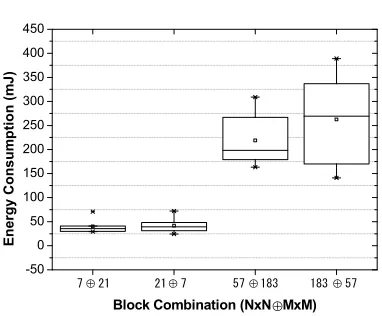
Figure 5 and Figure 6 show the simulation results of 10% and 1% duty cycles regarding latency and energy consumption. The graphs show that when the size of the front block combination is smaller than the reverse block combination such as and , its block combination is better than the reverse block combinations. Therefore, to get better performance, we must also consider block construction directions when combining block designs.

C2 C3 C4 C5

0 200 400 600 800 1000 1200 1400 1600 1800

Block Combination (Cn)

En

er

gy

C

on

su

mptio

n

(

m

J)

C2 C3 C4 C5

0 50 100 150 200 250 300 350

Block Combination (Cn)

Latency

518 Figure 5: Average latency of 10% and 1% back and

forward block combinations

Figure 6: Energy Consumption of 10% and 1% back and forward block combinations

6. SIMULATION RESULTS

To evaluate the effectiveness of EBNDP, we built a TOSSIM simulator using nesC and powerTOSSIM [9] in TinyOS [10]. For radio communications, sensor nodes use the CC2420 radio module [11]. The channel access scheme is based on CSMA/CA, and we apply a link model proposed by the ANRG group of USC [12] to our simulation study. For the simulation network topology, we assume 60 sensor nodes randomly deployed within a 100 m x 100 m ground area. To analyze simulation results, we consider simulation metrics such as latency and energy consumption.

In this paper, we assume following assumptions. All sensor nodes have a CC2420 radio module to exchange data packets between sensor nodes and perform bi-directional communication. Therefore,

if the sender sends a message to receiver sensor nodes, the receiver sensor nodes can respond to the sender with an ack message. Each sensor node performs communication during the phase of neighbor finding at the fixed location when it is deployed in the field at network initial time without mobility function. Their communication radius is about 100m. We assume that all sensor nodes exist in the communication radius range. We have also assumed that sensor nodes retransmit data if sensor nodes drop their packets.

Table 3 shows the overview of experimental environment.

Table 3: The parameters for experimental environmental

Properties Values

Network Topology Randomly topology

Experimental Area (100 100m ground area

Radio Module CC2420

The number of sensors 60

Event Trigger Time 15ms

Energy Calculator

Module PowerTOSSIM Module

Link Layer Model USC Link Model

Channel Access Scheme CSMA/CA

Radio Propagation Model Log-Distance Path Loss Model

Neighbor Discovery Protocols

Optimal, Random, EBNDP, Quroum, OR-based NDP

First, we study the relationship between duty cycles and latency distributions. It is evident that the length of block combinations increases as the duty cycle of sensor nodes decreases. This tendency can also be observed in the sample block combinations listed in Table 4.

Table 4: Block Combination Designs Selected By EBNDP Block Combination

7 7 ⊕ 21 21 147 10%

7 7 ⊕ 73 73 511 5%

31 31 ⊕ 91 91 2821 2%

57 57 ⊕ 183 183 10431 1%

Therefore, as shown in Figure 7, the latency distribution of NDS with a 1% duty cycle is much wider than in other cases. This means that to minimize the deviation of latency distributions, we must select a short block combination. That is why the proposed EBNDP algorithm puts more -20

0 20 40 60 80 100 120 140 160

57 183 183

57 7

21 21

7

Block Combination (NxN MxM)

L

aten

cy

(s

)



-50 0 50 100 150 200 250 300 350 400 450

 Block Combination (NxN MxM)

E

n

er

g

y C

on

su

m

p

ti

on

(m

J)

21

519 emphasis on the length of block combinations during the selection of the best candidate from the set T.

Figure 7: Relationship graph between duty cycles and latencies

Figure 8 shows the experiment results for 1 to 4 neighbors. If sensor nodes have only one neighbor, they just find one sensor node within their communication range. If a sensor node has four neighbors, it continually searches until the four neighbors are found. In Figure 8, as expected, the sensor nodes with only one neighbor have lower latency than others with 2, 3, or 4 neighbors. Furthermore, the sensor nodes with fewer neighbors have relatively lower latency deviation than others.

Figure 8: The discovery latency of the 1, 2, 3, and 4 neighbors on EBNDP algorithm

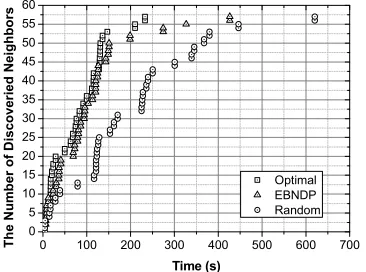
In Figure 9, we analyze the discovery time of neighbor sensor nodes for each NDP. The graph’s x-axis is the time, and its y-axis is the number of found neighbor nodes. Through this experimental

result, we show that EBNDP has lower latency than other NDPs at the same duty cycle. The main reason for this is that the total length of EBNDP is shorter than that of others within one cycle.

Figure 9: Relationship graph between duty cycles and latencies

Figure 10 and Figure 11 show the latency in HDC and LDC for each block design such as EBNDP, BIBD, and Random. In Random, we consider the worst-case block design among EBNDP block combinations at the same duty cycle. In the graph, we draw theoretical lines depending on packet drops as follows:

1 (2)

where k is a prime number, a time is the time

from start to end, and drop packets means the number of packet drops at particular duty cycles. For example, if k has a value of 9, a slot time is

15ms, and the drop packets are 2, then the latency can be calculated as follows:

9 9 1 15 2 2730 (3)

As shown in Figure 10, the latency of BIBD is close to the line of drop packets between 2 and 3. EBNDP also has a similar result as BIBD and is on the line of drop packet 3. Random is close to the optimal line of drop packet 4.

From these results, we know that BIBD has the best performance, EBNDP has better performance than Random by about one cycle length, but performance is slightly lower than Optimal.

10% 5% 2% 1%

0 20 40 60 80 100 120 140

Duty Cycle (%)

La

te

nc

y

(s

)

1 2 3 4

0 100 200 300 400 500 600 700 800

The Number of Neighbors

La

te

ncy

(

s)

0 100 200 300 400 500 600 700 0

5 10 15 20 25 30 35 40 45 50 55 60

Optimal EBNDP Random

Th

e

N

u

m

b

er

o

f

D

iscove

ri

ed

N

ei

gh

bor

s

520 Figure 10: Optimal vs EBNDP vs Random latencies in

HDC

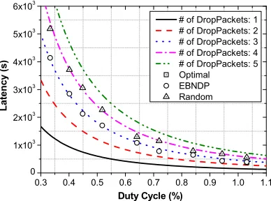
In Figure 11, we omit the result of BIBD because it cannot have any duty cycles under 1% due to its lack of duty cycle sets and because it has no block generating scheme. However, EBNDP and Random can easily generate block combinations with LDC.

In experimental results, we know that EBNDP’s latency is similar to # of DropPackets 3. On the other hands, latency of Random has similar to # of DropPackets 4.

Therefore, the performance of the EBNDP algorithm is better than randomly selected block designs.

Figure 11: Optimal vs EBNDP vs Random latencies in LCD

Finally, we compare EBNDP with other NDPs such as Quorum, Optimal, Random, and OR-based NDPs in asynchronous WSNs and symmetric duty cycles. The experiment reveals that Optimal,

OR-based, and EBNDP have similar latencies and that random NDP is worse than EBNDP and better than Quorum NDP as Figure 12.

However, note that BIBD and OR-based NDP cannot support various duty cycles in HWSNs. On the other hands, EBNDP can cover all the requirements of HWSN applications which require diverse duty cycles.

Therefore, we prove that EBNDP has similar performance to Optimal NDP and supports lots of duty cycles in HWSNs.

Figure 12: Latency Comparison of NDPs each duty cycle

In this paper, we introduced block combination scheme to support a variety of duty cycles. Moreover, in order to compare the performance of diverse block combination, we analyzed experimental results according to the number of block combination and combination direction. Furthermore, we showed latency depending on the number of neighbor sensor nodes.

In terms of the number of block combination, the latency of low block combination is better than high block combination although duty cycles are same. The reason is that high block combination reduces the ratio of sensor discovery due to the sparse common active point within long total cycle length. Therefore, if sensor nodes use EBNDP for their scheduling, low combination block should be used for low latency.

In terms of the combination direction, the direction from high duty cycle to low duty cycle is better than direction from low duty cycle to the high duty cycle. Especially, in this paper, we

2 3 4 5 6 7 8 9 10 11

0 10 20 30 40 50 60 70 80 90 100 110 120 130 140

La

tenc

y

(s)

Duty Cycle (%)

# of DropPackets: 1 # of DropPackets: 2 # of DropPackets: 3 # of DropPackets: 4 # of DropPackets: 5 Optimal

EBNDP Random

0.3 0.4 0.5 0.6 0.7 0.8 0.9 1.0 1.1 0

1x103

2x103

3x103

4x103

5x103

6x103

L

a

ten

cy

(s)

Duty Cycle (%)

# of DropPackets: 1 # of DropPackets: 2 # of DropPackets: 3 # of DropPackets: 4 # of DropPackets: 5 Optimal

EBNDP Random

1 2 3 4 5 6 7 8 9 10

0 50 100 150 200 250

La

te

ncy

(s)

521 considered 10% and 1% duty cycle to compare the performance of NDPs. Experimental results showed that direction from high duty cycle to low duty cycle has lower latency than another direction. The main reason is not accurate, but it is expected that the positions of the active slots of the high duty cycle are denser than the positions of the active slots of the low duty cycle.

In terms of the number of neighbor sensor nodes, as the number of neighboring sensor nodes increases, latency also increases at the similar rate. The main reason is that message collision is more likely to find the neighbor sensor, where there are many sensor nodes. That is, if sensor nodes drop neighbor discovery message to find their neighbors, they will have to wait until the next cycle. For this reason, latency is not good if there are many neighbor sensor nodes.

Therefore, if sensor nodes use EBNDP for their scheduling, we must consider several block combination features such as the number of block combination, block combination direction, and the number of neighbor sensor nodes. If we create new sensor nodes scheduling while keeping these block combination features, we can not only solve the disadvantages of BIBD but also provide similar performance to BIBD.

7. CONCLUSIONS

Neighbor discovery protocols are one of the critical issues in wireless sensor networks. The ultimate goal is to reduce latency and energy consumption. To support HWSNs applications, we must consider diverse duty cycles. In this paper, we introduced a new approach for constructing a block schedule for NDPs and proposed an effective block combination selection scheme called EBNDP to address the limitation of block design-based NDPs. EBNDP can generate various block designs depending on application requirements.

It is possible to provide various duty cycles through block combination scheme. However, we must consider some characteristics when blocks are combined. The reason is that although various combined sets can have the same duty cycle, they do not have the same performance.

In other words, different block combination can have the similar duty cycle, but do not have same active pattern within one cycle. It brings other performance. In this paper, we show that low block

combination scheduling is better than high block combination scheduling in terms of latency.

Similar to the number of block combination, although duty cycle is same, block combination direction can be different. In this case, we consider two cases such as the direction from high duty cycle to low duty cycle or direction from low duty cycle to high duty cycle. In this paper, though experimental results, we show that direction of the high duty cycle to low duty cycle is better than the direction of the low duty cycle to the high duty cycle.

In this paper, we constructed an experimental environment based on the TOSSIM simulator, which is a sensor network simulator. In order for the simulation environment to resemble the HWSN, we put representative the wireless channel model and the channel access scheme into TOSSIM simulator. We compare the performance of EBNDP with other NDPs such as optimal, random, Quorum-based NDP, and OR-based NDP. Through various experimental results, we prove that EBNDP has better performance than other NDPs.

In this paper, we show basic concept to combine block design-based NDPs for sensor scheduling. It can be used for diverse fields such as security, artificial intelligence, sensor transmission power control and IoT platform.

In future works, we will extend block combination scheme to support both symmetric and asymmetric duty cycles and take additional experiments considering real-world objects. Moreover, we plan to integrate our combination method with the IoT platform to provide various IoT service models such Healthcare, U-Transportation, and U-City. Finally, we plan to build a large system that can perform intelligent analysis by linking the concept of artificial intelligence with our future system.

ACKNOWLEDGMENTS:

This research was supported by Basic Science Research Program through the National Research Foundation of Korea(NRF) funded by the Ministry of Education(NRF-2015R1D1A1A01058786)

REFERENCES:

522 [2] Zheng, R., Hou, J.C. and Sha, L., Asynchronous

Wakeup for Ad Hoc Networks, In Proceedings of the 4th ACM International Symposium on Mobile Ad Hoc Networking &Computing, (2003), 35-45.

[3] Lee, W.S., Choi, S.G., Song, T.S., Kim, N.G. and Youn, J.H., OR-based Block Combination for Asynchronous Asymmetric Neighbor Discovery Protocol, International Journal of Control and Automation, 8 (2015), 45-52. [4] Choi, S.G., Lee, W.S., Youn, J.H., Dreizan, M.

and Matthew, S., An Energy-Efficient Neighbor Discovery Protocol for 6LoWPAN Smart Grid Applications, IEEE WCNC 2015, (2015), 52-57.

[5] Lee, W.S., Choi, S.G., Kim, N.G., Youn, J.H. and Dreizan, M., Block Combination Selection Scheme for Neighbor Discovery Protocol, IEEE CSNT 2015, (2015), 143-147.

[6] Jiang, J., Tseng, Y., Hsu, C. and Lai, T., Quorum-based Asynchronous Power-saving Protocols for IEEE 802.11 Ad Hoc Networks, Mob.Netw.Appl., 10 (2005), 169-181.

[7] Shrestha, N., Youn, J.H. and Sharama, N., A Code-Based Sleep and Wakeup Scheduling Protocol for Low Duty Cycle Sensor Networks, Journal of Advances in Computer Networks, 2 (2014), 80-85.

[8] Kandhalu, A., Lakshmanan, K. and Rajkumar, R., U-Connect: A Low-latency Energy-efficient Asynchronous Neighbor Discovery Protocol, in Proceedings of the 9th ACM/IEEE International Conference on Information Processing in Sensor Networks, (2010), 350-361.

[9] Perla, E., Cathain, A.O., Carbajo, R.S., Huggard, M. and Goldrick, C.M., PowerTOSSIM Z: Realistic Energy Modelling for Wireless Sensor Network Environments, the 3nd ACM Workshop on Performance Monitoring and Measurement of Heterogeneous Wireless and Wired Networks, (2008), 35-42. [10] Levis, P., Lee, N., Welsh, M. and Culler, D.,

TOSSIM: Accurate and Scalable Simulation of Entire TinyOS Applications, in Proceedings of the 1st International Conference on Embedded Networked Sensor Systems, (2003), 126-137. [11] CC2420 Data Sheet, [Online]. Available:

https://inst.eecs.berkeley.edu/~cs150/Docume nts/CC2420.pdf

[12] USC Link Model, [Online]. Available:

http://www.tinyos.net/tinyos-2.x/doc/html/tutorial/usc-topologies.html