CLASSIFYING ARABIC TEXT USING DEEP LEARNING

3608

MODELING AND QUERYING SPATIOTEMPORAL

MULTIDIMENSIONAL DATA ON SEMANTIC WEB:

A SURVEY

1,2 _{IRYA WISNUBHADRA,} 3_{SAFIZA SUHANA KAMAL BAHARIN,} 4_{NANNA SURYANA}

HERMAN

1 _{Department of Informatics Engineering, Universitas Atma Jaya Yogyakarta, Indonesia}

2,3,4 _{Centre for Advanced Computing Technology, Fakulti Teknologi Maklumat dan Komunikasi, Universiti}

Teknikal Malaysia Melaka, Malaysia

ABSTRACT

The usage of “web of data” for decision making has increased with the presence of On-Line Analytical Processing (OLAP), Data Warehouse (DW), Multidimensional Data (MD), and Semantic Web (SW) technologies. These technologies are converging into technology that utilizes data on the web to obtain important information as the basis of crucial decision making. The implementation of these technologies continues to grow along with data published on the web using vocabularies like SDMX, QB, and QB4OLAP for linked cube data. Along with increasing analysis complexity, spatiotemporal OLAP emerges as a tool to obtain sophisticated, better, and more intuitive analysis results than OLAP. Vocabulary for spatial OLAP on the Semantic Web has been constructed, namely QB4SOLAP, and successfully implemented. Query language extension for SW was built significantly, but the fundamental model of more dynamic spatial (spatiotemporal) multidimensional data for OLAP on the SW still lacks to exhibit and implemented, even Spatiotemporal DW has been widely studied. This paper presents state-of-the-art research results and outlines future research challenges in Spatiotemporal multidimensional data on the semantic web. This paper organized into three parts, the first part (1) discusses the convergence of OLAP / DW and SW, the second part (2) discusses DW, and spatiotemporal DW on the SW based on the model and the query, and (3) discusses future research opportunities.

Keywords: Spatiotemporal, Multidimensional Data, Semantic Web, Modeling, Querying

1 INTRODUCTION

Business Intelligence (BI) is a technology for collecting, transforming, and presenting data for analysis as a tool for supporting decision making. BI uses Data Warehouse (DW), Multidimensional (MD) data, and Online Analytical Processing (OLAP) that has proven to be useful for obtaining information and knowledge relevant to the business [1]. A Data Warehouse (DW) is a tool that gathers, transforms, and loads data from transactional databases and external sources to provide information to decision-makers. DW has to be maintained in a consistent and consolidated method. The technologies related to DW is OLAP multidimensional (MD) data processing. MD models defined observation as a fact and dimension in a star or snowflake scheme table and queried using de facto standard language Multi-Dimensional Expression (MDX). BI technology has been widely

adopted by proprietary or open-source software and massively used by organizations.

ISSN: 1992-8645 www.jatit.org E-ISSN: 1817-3195

3609 which then generates Semantic Linked Data (e.g: Linked Data, Linked Open Data, and Government Linked Open Data). The availability of the web of data can be access using query language named SPARQL with its endpoint.

Business and Government have published their data in SW with an open concept, which produces large amounts of valuable data in the form of semi-structured data, flexible and machine-readable. Impressive examples are Dbpedia [4], data.gov, geonames, and data.gov.uk. The field of health and life science is also massively utilizes linked data, namely: UMLS [5], SNOMED-CT, GALEN, GO, Bio2RDF, Linked Life Data, and Linking Open Drug Data. They launch an open data portal to provide data access as statistical data [6]. The statistical data have multidimensional characteristics.

In the modern and competing environment, there is an urgent requirement of tools that able to exploit, analyze, and summarize all statistical data from “web of data” resources. The exploitation of a statistical web of data became popular in the last few years. The government institutions has published their statistical data using cube vocabulary, and has reach 61.75% of their domain. Consequently, many developments focused on using, validating, and visualizing this statistical datasets [7]. Many researchers have been work intensively to implement the concept of BI on the SW. Implementation BI on the SW has many issues, the first issue is OLAP modeling on the SW, the second is the integration process from disperse data source to the DW, and the last issue is data access using query language. Moreover, some researchers worked with system architecture and implementation, user interface design, dataset, and applications of the SW for BI.

Along with increasing analysis complexity, spatiotemporal OLAP emerges as a tool to obtain better and more intuitive analysis results than OLAP. Spatiotemporal OLAP is a combination of GIS and OLAP that could handle spatial data objects, temporal data objects, temporal-spatial types or moving objects and evolving data warehouse

dimensions. An enormous volume of

geographic/spatial data has been published using SW, yielding the need for Spatial OLAP for analysis spatial or non-spatial data. Spatial OLAP has been

modeled on SW by QB4SOLAP vocabulary, which supports spatial operators and algorithms for spatial aggregate SPARQL querying [8].

Although, the research on spatiotemporal OLAP/DW or moving objects have been attracted to many researchers in the last decade because of the wide availability of devices that track the position of moving objects, modeling and querying spatiotemporal OLAP on the SW still lack the significant foundation of treatment. Deep analytic support for spatiotemporal OLAP on SW data is very valuable, it needs modeling and querying that consist of function, methods, manipulation techniques, and vocabulary representing spatiotemporal data warehouse, that is still not available today.

1.1 Paper Contribution

Firstly, the paper presents the background of the importance of modeling and querying spatiotemporal multidimensional data on SW. Secondly, the paper presents the survey strategy and then describes the characteristics of DW/OLAP and SW, the convergence of DW and SW, and the approach of combining DW and SW. Then, the paper describes modeling and querying multidimensional data, both from the conventional OLAP DW to the Semantic Linked Cube Data, and makes a comparison of modeling and querying features of DW that have been implemented on the SW. The next section will be discussed the conceptual model of spatiotemporal DW, and findings from the modeling and querying spatiotemporal multidimensional data on the SW. Finally, all the discoveries are discussed and several guidelines for prospect research are defined.

2 SURVEY STRATEGY

Survey strategy is important in the survey to guarantee the breadth and depth of the studies. The survey strategy consists of three steps:

a) Identification of Research Questions (RQ) b) Digital library selection

c) Search string identification

2.1 Identification of Research Questions

3610 identified to support this survey, as presented in table 1.

Table 1. Research Question

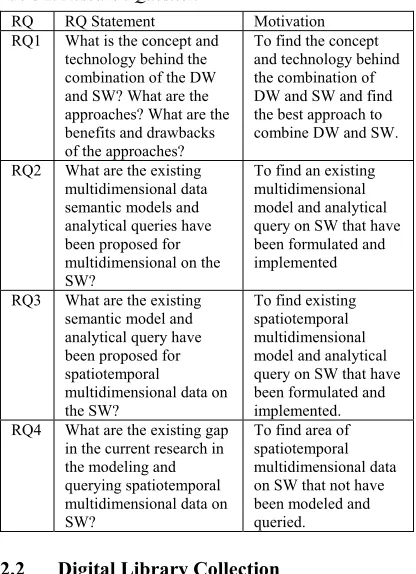
RQ RQ Statement Motivation RQ1 What is the concept and

technology behind the combination of the DW and SW? What are the approaches? What are the benefits and drawbacks of the approaches?

To find the concept and technology behind the combination of DW and SW and find the best approach to combine DW and SW. RQ2 What are the existing

multidimensional data semantic models and analytical queries have been proposed for multidimensional on the SW?

To find an existing multidimensional model and analytical query on SW that have been formulated and implemented RQ3 What are the existing

semantic model and analytical query have been proposed for spatiotemporal

multidimensional data on the SW?

To find existing spatiotemporal multidimensional model and analytical query on SW that have been formulated and implemented. RQ4 What are the existing gap

in the current research in the modeling and querying spatiotemporal multidimensional data on SW?

To find area of spatiotemporal multidimensional data on SW that not have been modeled and queried.

2.2 Digital Library Collection

The selection process is started with entering ‘Data Warehouses’ and ‘Semantic Web’ between 2010 – 2019 as search strings on Google Scholar repository. This query results from 4.010 of papers and filtered from several popular databases research area to collect the primary papers originated from recognized databases. The popular databases are:

a) Springer b) Science Direct c) IEEEXplore d) EmeraldInsight e) Taylor & Francis f) ACM Digital Library g) Wiley Online Library

2.3 Search String Identification

The authors search papers from the digital library collection with search string ‘Data Warehouses’ and ‘Semantic Web’ between the year 2010 until 2019 with the language exclusion not in English. The results of the query are depicted in figure 1.

Figure 1. Search string query and the results

Table 2. Inclusion dan Exclusion Criteria

Inclusion Criteria Exclusion Criteria Using the English

Language

Not Using the English Language

Paper related to Modeling and Querying

Multidimensional data on SW

Identical papers

Paper is related to at least

one research question Paper does not relate to research questions Paper is peer-reviewed in

journals, conferences, or workshops

Paper is not peer-reviewed, presentations

The result of applying inclusion, exclusion, and snowball technique are 80 papers are fit to answer all the research question defined earlier.

3 BUSINESS INTELLIGENCE AND

SEMANTIC WEB

ISSN: 1992-8645 www.jatit.org E-ISSN: 1817-3195

3611 quality and complete data, but the completeness might not be obtained only from internal databases, so that BI has to link to external data, such as competitor data, markets, potential buyers, government rules, and politics [9].

BI grows with the capability to adapt to external data sources that have an unstructured, semi-structured, and flexible format. BI grows its scope that extends to not only strategic decision support but also the tactical decision that makes new terms like BI 2.0 [10], on-demand BI, Self Service BI [11], and fusion cube [12].

Furthermore, the exploratory OLAP concept emerges as a BI that has the ability to explore and access new data sources with new data structures, to store new data, and to query these new data [13], [14]. One of the technologies behind the Exploratory OLAP is the Semantic Web. This technology becomes mature. SW allows data sharing in a dynamic way, publishing data and linking semi-structured data on the web using standards, besides SW also has the ability to support inferencing and active reasoning. In order to support the data sharing process, SW has accurate and rich data declarations through ontology and vocabulary. SW also supports efficient data acquisition with SPARQL. Data integration with SW is supported by the ability to provide data meaning that it is indispensable for the process of cleansing, merge, and combining data from a variety of sources to become multidimensional data. The process of analyzing data through queries is also equipped with the ability to give meaning to data not only for results but also where the data comes from. 

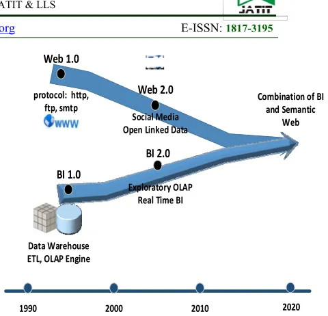
Over several years, the direction of BI and SW research has been different, but in the last decade research in these two domains shows us the convergence and the mutually beneficial. BI proposed sophisticated tools for analyzing the huge amount of data with an outstanding performance, whereas SW linked data proposes an exploratory opportunity of valuable information that could be used for enriching business analytics with inferencing capability [12], [15]–[19]. The convergence of the BI and SW showed in figure 1.

BI 1.0 Web 1.0

BI 2.0 Web 2.0

Exploratory OLAP Real Time BI

Data Warehouse ETL, OLAP Engine 

Social Media Open Linked Data protocol:  http, 

ftp, smtp Combination of BI and Semantic  Web

1990 2000 2010 2020

Figure 2. The convergence of Business Intelligence and

Semantic Web research direction 

Developing OLAP using SW categorized into three types of approaches, the first approach is an integration-based approach that focuses on data source integration, the second is an analysis-based approach that focuses on analytical processing and the third is a combination of these two approaches. A detailed discussion of the three approaches is as follows:

3.1 The integration-based approach

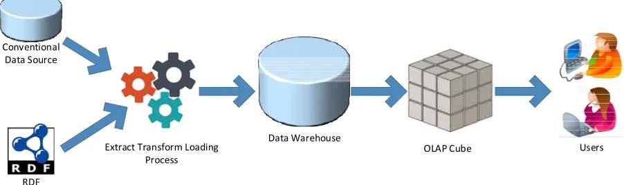
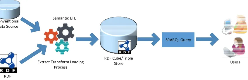
An integration-based approach is an approach that focuses on the process of extracting, transforming, and loading (ETL), from RDF data sources to DW. The integration-based approach has been proposed because RDF data does not have a data structure that allows OLAP operations to be imposed on it, such as: drill down, roll up, slice, dice, etc. The ETL results are stored in a multidimensional cube that can be easily accessed using MDX query language for analysis. This approach is also known as a schema-on-write approach where requires a multi-dimensional schema to be designed and the ETL process to be set as a write process before the query is executed. The illustration of this concept is shown in figure 2. The ETL process input is coming from the data source that may have a different format, semantic or non-semantic data. ETL process will build DW and Cube that OLAP operations could be used to support analysis.

3612 DW warehouses originating from single domain ontology representing multiple heterogeneous data sources from many business domains [20]. Furthermore, research by Niinimaki et al. developed a technique to practice ontology and mapping files that connect to the data sources from external sources with the ontology. Then, the ETL process is performed according to the ontology and mapping files. OLAP ontology defines measures and dimensions using Ontology Web Language (OWL) and Resource Description Framework (RDF). This research-validated by performance testing using 450,000 RDF statements and give outstanding performance [21]. Likewise, Nebot et al. suggest a solution to solve the problem of combining DW and SW technologies. They proposed a framework for designing a model of MD analysis with the semantic annotation stored in a Semantic DW (SDW) that stores web resources, domain ontologies and the semantic annotations using XML. Their finding claims has a new semi-automatic approach to defining multiple domain ontology, scalable, and well formalized [22]. Additionally, Jiang et al.proposed a method to handle data heterogeneity to build DW with the domain ontology in the integration process. Domain ontology has created using classes of Web Ontology Language and inserted in the metadata of the DW that could describe the logic of transforming data, discover the data sources, and remove the heterogeneity. The

method has been implemented in a hospital DW, and medical domain ontology plays an important role [23]. Likewise, Bergamaschi et al. developed an ETL tool that could support semantic mappings from the data source with inter-attribute definition to support the extraction and transformation process to the DW schema. The tool has been implemented for developing DW in the case of the food and beverage logistics area and resulting effective method [24].

Moreover, Kampgen et al. proposed a concept of integrating multiple Linked Data sources of statistical data. Their research created a design to convert from Linked Data into the Cube model in DW, then execute the design using an ETL pipeline process, and thus load the conversion results into an open-source OLAP system. This research also shows how the infrastructure of OLAP could be used for querying and visualizing integrated statistical Linked Data [15]. Inoue et al. developed a general ETL framework for Linked Open Data (LOD) dataset. Their framework can execute the ETL process to the datasets regardless of the usage of the OLAP Cube vocabulary and could explore semantic hierarchies in the dataset even from external LOD such as geonames and DBpedia [25]. Further, An ETL-based approach is developed in the H-SPOOL framework that does extract OLAP- related information from SPARQL endpoints that have the advantage of reducing the number of downloaded triples [26].

Figure 3. Integration-Based OLAP On Semantic Web Architecture

The integration-based approach has the advantage of the usage of mature and proven OLAP technology, on the contrary, this method still has disadvantages that the refreshment process of LOD data to DW still performed in semi-automatically way, making it difficult to maintain consistency

between data warehouse and online data for analysis purposes.

3.2 The analysis-based approach

This approach focuses on analytical processes that carried out directly on Semantic Web / RDF data without the ETL process. In this approach, Data Warehouse

Extract Transform Loading  Process

Users Conventional 

Data Source

RDF Data Source

ISSN: 1992-8645 www.jatit.org E-ISSN: 1817-3195

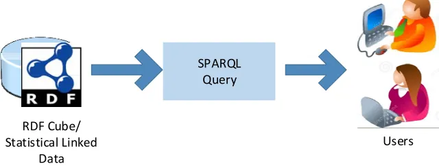
3613 multidimensional data requires vocabulary to model data cubes, dimensions, and measures in RDF. This approach sometimes called a schema-on-read approach. The de facto standard of vocabulary for RDF Data Cube is QB1_{. Many proposals have been}

successfully explored this approach. Firstly, Kampgen et al. define a proposal to model querying statistical Linked Data using common OLAP operations on RDF data cubes. This research also found a set of OLAP query functions and operators using SPARQL language. Both models and queries are executed directly on a triple repository without intermediate storage; therefore, if the RDF is changed, modifications are disseminated to OLAP clients. This research also improved the QB vocabulary for enhancing multidimensional statistical data representations [27].

Moreover, Etcheverry and Vaisman developed Open Cube (OC) vocabulary that using RDFS for publishing multidimensional cubes on the SW. Using Open Cube, traditional OLAP operations possibly executed using SPARQL 1.1., and web cube could be mapped to the multidimensional model in order to be able to operate with the local cubes. OC also developed to support model with dimensions with multiple hierarchies, but OC has a disadvantage that could not reuse QB vocabulary that has been used before [28]. 

Saad et al. create an efficient RDF constellation model by proposing a formalization of multidimensional structure. This model supports multiple facts, multiple dimensions, and multiple hierarchies. Based on this formalization, operators of OLAP can be interpreted into SPARQL queries that comply with the constellation model [29]. Furthermore, Ibragimov et al. developed a framework called Exploratory OLAP over RDF sources. This research proposes a system using RDF vocabularies to define OLAP cube with a multidimensional schema. The system is intelligently executing the query to extract and summarize data, and also build a cube based on the vocabularies. This project also creates a process for determining unidentified data sources and constructing a multidimensional schema of the cube. In this approach, vocabulary for multidimensional or statistical data is an important issue because OLAP in the semantic web requires complex models for the fact, dimension, level, hierarchy, etc. [18].

Moreover, the research conducted by Etcheverry develop an extension of QB that models multidimensional data with the new vocabulary; it is called QB4OLAP. QB4OLAP supports balanced hierarchy, recursive, ragged, and many-to-many relationships that most used on the multidimensional model.

Users RDF Cube/ 

Statistical Linked  Data

SPARQL  Query

Figure 4. Analysis-based Architecture OLAP on Semantic Web

This research also suggested a mechanism to translate a multidimensional model into QB4OLAP vocabulary’s RDF file and proposed a transformation of relational DW into the QB4OLAP model using a translator, R2RML. The QB4OLAP cubes could be accessed using SPARQL [30]. Additionally, QB4OLAP made an extension of the QB RDF Data Cube for modeling multiple levels of dimensions and aggregate function.

3614 SPARQL queries (MARVEL). Many application tools have been built using this approach and used by government and industries, e.g. http://opengovintelligence.eu, which continues to develop, expanding, and exploiting Statistical Linked Open Data, with the TARQL extension, and D2DQ, called the Linked Open Cube Analytics (LOCA) system [32]. On the other hand, Boumhidi et al.proposed a method for directly querying the cube data stored modeled by QB vocabulary with an interactive OLAP via MDX to SPARQL mapping without any materialization. This research also constructed a formal algebra of OLAP operations on data cubes published as Linked Data [33].

This analysis-based approach described earlier, actually overcomes the problems of the previous integration-based approach on the issue of ETL and data refreshment. The analysis-based approach provides multidimensional OLAP modeling that is suitable for Linked Data but the impressive materialization and pre-aggregation aspects of the cube on linked data still left a problem to be solved.

3.3 The combination approach

This approach is fully integrated SW in all layers of BI. It had been known, one of the

drawbacks of the implementation of the integration-based approach is that the ETL process for the linked data source traditionally prioritizing data schema. This method is considered ineffective because Linked Data has a schema-dependent nature, or sometimes has a complex schema, or even only have an implicit schema. Data on SW may have a condition where different sources can explain the same data in different ways. The integration of data for heterogeneous data using semantic data is a necessity that cannot be avoided. This combination approach improves the weaknesses of traditional ETL that fully integrate the Semantic Web with the Data Warehouse, in this way the BI community benefits from the analysis process with semantically annotated data. Several researchers proposed this combination approach, among them, are Colazzo et al. proposed a bottom-up redesign of the core data analytics concepts and tools, on RDF data. This design is fitted with Linked Data with rich semantic and heterogeneous format. This design using a full RDF warehousing approach, where the data source and the DW are in RDF graph format. This research also defines analytical schema and queries and optimization techniques with schema materialization [34].

RDF Cube/Triple  Store Extract Transform Loading 

Process

Users Conventional 

Data Source

RDF Data Source

SPARQL Query Semantic ETL

Figure 5. The combination between integration-based and analysis-based Architecture OLAP on Semantic Web

Moreover, Bansal and Kagemann researched to create ETL tools that are able to integrate data from various heterogeneous sources by utilizing semantic data to enrich the integration process [35]. Furthermore, Nath et al. proposed a programmable framework called Semantic ET (SETL) that could support the development of Semantic Data Warehouse. SETL using TBox and QB4OLAP

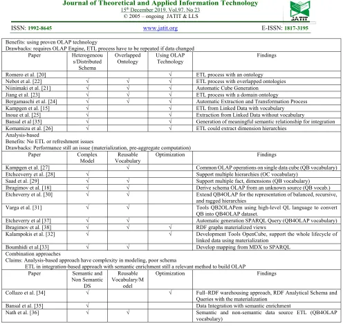
schema to create Multidimensional data for Semantic and Non-Semantic Data Source [36]. Table 3 shows the summary of the OLAP development using the SW. The comparison, benefits, and drawbacks of the three approaches have described in this table.

Table 3. Summary of OLAP development using Semantic Web

ISSN: 1992-8645 www.jatit.org E-ISSN: 1817-3195

3615

Benefits: using proven OLAP technology

Drawbacks: requires OLAP Engine, ETL process have to be repeated if data changed Paper Heterogeneou

s/Distributed Schema

Overlapped Ontology

Using OLAP Technology

Findings

Romero et al. [20] √ ETL process with an ontology

Nebot et al. [22] √ √ √ ETL process with overlapped ontologies Niinimaki et al. [21] √ √ √ Automatic Cube Generation

Jiang et al. [23] √ √ √ ETL process with a domain ontology

Bergamaschi et al. [24] √ √ √ Automatic Extraction and Transformation Process Kampgen et al. [15] √ √ ETL from Linked Data with vocabulary Inoue et al. [25] √ √ Extraction from Linked Data without vocabulary

Bansal et al [35] √ √ Generation of meaningful semantic relationship for integration Komamizu et al. [26] √ √ ETL could extract dimension hierarchies

Analysis-based

Benefits: No ETL or refreshment issues

Drawbacks: Performance still an issue (materialization, pre-aggregate computation) Paper Complex

Model

Reusable Vocabulary

Optimization Findings

Kampgen et al. [27] √ Common OLAP operations on single data cube (QB vocabulary) Etchceverry et al. [28] √ Support multiple hierarchies (OC vocabulary)

Saad et al. [29] √ √ Support multiple fact, dimensions (QB vocabulary) Ibragimov et al. [18] √ √ Derive schema OLAP from an unknown source (QB vocab.) Etcheverry et al. [30] √ √ Extend QB4OLAP for the representation of balanced, recursive,

and ragged hierarchies

Varga et al. [31] √ √ Tools QB2OLAPem using high-level QL language to convert QB into QB4OLAP dataset.

Etcheverry et al [37] √ √ Automatic generation SPARQL Query (QB4OLAP vocabulary) Ibragimov et al. [38] √ √ √ RDF graphs materialized views

Kalampokis et al. [32] √ √ Development Tools OpenCube, support the whole lifecycle of linked data using materialization

Boumhidi et al.[33] √ √ Develop mapping from MDX to SPARQL Combination approaches

Claims: Analysis-based approach have complexity in modeling, poor schema

ETL in integration-based approach with semantic enrichment still a relevant method to build OLAP Paper Semantic and

Non Semantic DS

Reusable Vocabulary/M

odel

Optimization Findings

Collazo et al. [34] √ √ Full–RDF warehousing approach, RDF Analytical Schema and Queries with the materialization

Bansal et al. [35] √ Data Integration with semantic enrichment

Nath et al. [36] √ √ Semantic and non-semantic data source ETL (QB4OLAP vocabulary)

4 MULTIDIMENSIONAL DATA MODEL

The multidimensional data model or a data cube was introduced as an infrastructure of OLAP and DW. The concept of OLAP popularized by Codd [39] as a method of executing complex analysis over information stored in a DW. A DW is a considerable data repository with subject-oriented, integrated, time-variant, and non-volatile data organized specifically for analytical purposes [40]. A DW is designed in the form of a star schema or snowflake that has a fact table and dimension table. A DW is designed to be performed well by drill-down, roll-up, slice, and dice operations. The fact table contained cells associated with numerical values

called measures. The analysis process assesses many aspects of the business using these measures. For example, the cube of data in figure 6 shows a cell

3616 that represents a measure of Quantity, indicating the numbers of agriculture production (in thousands ton) by-product(category), time(quarter), and farmer(province). A data cube usually has several measures. For example, another measure on the agricultural cube, not shown in the figure, could be the total sales amount from agriculture production. The dimension table is a representation of a dimensional perspective of analysis. Dimension has levels and descriptors. For example, the data cube in figure 6 can be used to analyze production figures. The cube has three dimensions: Product, Time, and Farmer. A dimension level represents the detail level of the data and often called granularity. A level has attributes that describe the dimension. For example, the production cube is summarized to the levels Category, Quarter, and Province. Dimensions have instances called members, for example, Rice and Soybeans are members of the Product dimension at the Category level. Dimensions also have attributes to describe the characteristic of the dimensions. For example, the Product dimension could have attributes such as ProductId and PricePerKg.

In the concept of DW, the term hierarchy on the dimension is known, which enables decision-makers to get more detailed information for strategic analysis purposes. For example, in the data cube shown in fig 6, information on the quantity of production could be enhanced to the finer granularity in the month order, or the coarser granularity on the farmer dimension at the country level. The hierarchy will define the sequence of mapping that connects concepts from higher or more general concepts to lower or more detailed concepts. The hierarchy has many types, including balanced, unbalanced, multiple, recursive, generalized, alternative, and parallel hierarchies.

The hierarchy concept of the data cube related to the aggregation process of each measure in a data cube. The aggregation process performed by traversing to this hierarchy of the dimension. The aggregation process usually takes place when the user wants to visualize the aggregation of measure interactively by changing the level of detail of the dimension. For example, if we want to visualize data cube in figure 5 by Country, then we must to change granularity to the coarser detail from Province to Country, then the Production figures for all farmers in the same country will be aggregated using, for

example, the SUM operation. The measure can be categorized as follows:

a.The additive measure is a measure that could be aggregated using addition for all the dimensions, using addition. The additive measure is a common type of measure.

b.The semi-additive measure is a measure that could be meaningfully aggregated for some dimensions using addition. For example, a measure product inventory that summarized for two months didn’t give meaningful aggregation. c.The non-additive measure is a measure that

could not be meaningfully aggregated along any dimension. For example product price, and currency rate.

d.The derived measure is a measure derived from another measure.

4.1 OLAP Operations

The multidimensional model gives the environment that could interactively analyze data for descriptive information from multiple dimensions and at several levels of detail. The model using OLAP operators that could aggregate and materialize data along dimensions and hierarchies. The OLAP operators are:  

(a) Aggregate Function: a function that aggregate measure of a cube, including SUM, AVG, COUNT,

MIN, MAX, TOPPERCENT, BOTTOMPERCENT,

RANK, and DENSERANK. The syntax for the

aggregate function is:

AggFunction(Cube,Measure)[BY Dimension]

For example, from figure 5, total production by month and province could be expressed by

SUM(Production,Quantity) by TIME.MONTH, FARMER.PROVINCE

(b) ROLLUP: query to aggregates measures

alongside the hierarchy of dimensions using an aggregate function. This query acquires measures at a rougher granularity. The syntax of measures ROLLUP operation is:

ROLLUP(Cube,(Dimension→ Level),

AggFunction(Measure))

for example, total quantity by the month of production cube is:

ROLLUP(Production,(Time→ Month),

SUM(Quantity))

ISSN: 1992-8645 www.jatit.org E-ISSN: 1817-3195

3617 hierarchy itself; it is called the recursive hierarchy. ROLLUP operations will be varied

with recursive ROLLUP or RECROLLUP, the

syntax of recursive roll up is:

RECROLLUP(Cube,(Dimension→

Level),Hierarchy, AggFunction(Measure))

(c) SLICE: cut a cube for a certain dimension and

value. The syntax of slice operation is:

SLICE(CubeName, Dimension, Level

= Value))

for example, the total quantity of production in Banten province is:

SLICE(Production, Farmer, Province = ‘Banten’))

(d) DICE: get data from cube to obtain information

like dice in the cube, similar to the relational algebra of selection 𝜎 𝑅 , where p is the

boolean predicate conditions over-dimension levels, attributes, and measures. The syntax of dice operation is:

DICE(CubeName, p),

for example, total quantity by the month of production cube is:

DICE(Production,

(Farmer.Province = ‘Banten’ OR Farmer.Province = ‘East Java’) AND (Time.Month= ‘JAN’ OR Time.Month= ‘FEB’))

(e) DRILLDOWN: query to get more detailed data

from a deeper level in a hierarchy. The syntax of the drill-down operation is:

DRILLDOWN(CubeName,(Dimension→

Level))

for example, the total quantity by the quarter of the production cube is:

DRILLDOWN (Production, (Time→

Month))

(f) PIVOT: query to provide an alternative

presentation of data. The syntax of the pivot operation is:

PIVOT(CubeName,(Dimension→

Axis))

for example, the total quantity by a quarter of the production cube is:

PIVOT(Production,Time→

Quarter,Farmer→ Province,Product→

Category)

(g) DRILLACROSS: query to get data from the

combination of two common schema data cubes. DRILLACROSS query naturally has the

same operation with a full outer join in the relational algebra. The syntax of DrillAcross operation is:  

DRILLACROSS(CubeName1,CubeName2 ,Condition)

for example:

DRILLACROSS(Production,Producti on1, Production.Time.Month+1 = Production.Time.Month)

4.2 Linked Cube Data Model and Query

For publishing linked data cube/statistical data, the model of the cube data is a core foundation. The linked data cube model is represented by vocabulary. Many vocabularies have been developed to model multidimensional data with facts, dimensions, and hierarchies as RDF graphs and to query RDF graphs with OLAP operators. The first standard model of statistical data proposed by the International Organization for Standardization (ISO) in 2005, it is called the Statistical Data and Metadata Exchange (SDMX). The SDMX initialized by seven international institutions (UN, World Bank, IMF, Eurostat, BIS, and European Central Bank) with the purpose of improving efficiency and enhance quality using advance technology for share and exchange statistical data and metadata among institutions for interoperability. The SDMX covers how to represent statistical data in flat files and as XML to the definition of fact, dimension, and measure. SDMX

created under Content-Oriented Guidelines (COGs) that define a set of code lists, cross-domain concepts, and categories with the aim of delivering interoperability and compatibility across organizations. Many researchers have implemented the SDMX to publish statistic data and access the data using web services, and the advent of linked data makes SDMX could be modeled with the linked data that provide some benefits [41]. The design and implementation of SDMX-ML to RDF/XML using XSL transformations have implemented to publish linked data from Organization for Economic Cooperation and Development (OECD), Swiss Federal Statistical Office (BFS), Food and Agriculture Organizations of United Nations (FAO), European Central Bank (ECB), and International Monetary Fund (IMF) [42].

3618 framework for modeling and sharing, accessing, and publishing statistical data. But SCOVO has the disadvantage of did not have a feature of organizing the data into slice dataset, or notion of dimensions, measures, and attributes that different in structure [43].

Furthermore, statistical vocabulary standards have been proposed, the vocabulary is called the Simple Knowledge Organization System (SKOS) vocabulary. The SKOS models common features in a standard thesaurus using classes and properties. The vocabulary of the SKOS using a concept-centric view that explains abstract notions represented by terms, but primitive objects are not terms. Each SKOS concept is defined as an RDF resource that can have properties like index terms, synonym, definition, and notes. Concepts could be arranged in hierarchies using broader-narrower relationships, or connected by non-hierarchical relationship. Concepts grouped in concept schemes, containing a consistent and structured set of concept that create controlled vocabulary [44]. However, The SKOS vocabulary that relied on loosely defined notions of ‘broader than’, ‘narrower than’, and ‘related to’ relationships not rich enough to handle more complex hierarchical relations, e.g., generic-specific, whole-part, causal, sequential, and temporal relations. There is a need to extend the SKOS to handle these relations, and also statistical researcher requirements as well as requirements from ISO 704:2000 and ISO 1087-1:2000 standard.

The new vocabulary is called XKOS. Cotton et al. has been described XKOS in the journal paper including the concepts, structures, terms and codes, and associative relations. XKOS categorized data between the concepts and the real-world objects and make a relationship between them. XKOS is built to provide a reusable standard on the RDF for publishing statistical data available through new web technologies [45].

The new milestone in modeling linked cube data has emerged with the RDF Data Cube, QB vocabulary. QB adheres to linked data principles and the RDF model. It becomes a W3C standard for modeling data cubes. QB is based on the core components of the SDMX information model. QB could define the structure of the cube, cube, instance of the cube, measure, dimension, etc. The main class in the QB is qb:DataSet that provides a definition of

a cube. The qb:DataStructureDefinition describes

the cube’s data structure. The qb:Observation class

defines each cell of the cube as a measure. The vocabulary structure of QB is specified by the abstract class qb:Component- Property, that has

three sub-classes, namely qb:DimensionProperty

that describes the dimensions of the cube,

qb:MeasureProperty that defines measured

variables, and qb: AttributeProperty that defines the

structural metadata [46]. At this moment, 11.24% of the datasets as Linked Data Cubes use the QB vocabulary [47]. The advent of QB vocabulary makes linked data cube popular among organizations. Many organizations created link data cubes, for example, European Commission developed Digital Agenda Scoreboard as a visualization tool that built from linked data cubes, Eurostat transformed their research data to linked data cubes that includes more than 5000 data, and the publication of the linked data cubes of 2011 census data from Ireland, Greece and Netherland [48].

ISSN: 1992-8645 www.jatit.org E-ISSN: 1817-3195

3619 Furthermore, the researchers try to enhance the feasibility of a linked cube model with optimization. Colazzo et al. proposed analytical schema and queries using full RDF warehousing with schema materialization [34]. Azirani et al. proposed systematic optimization for efficient OLAP operations. His technique tries to solve the question of computing an Analytical Query based on the materialized answer of another Analytical Query [49].

The QB is becoming a W3C standard to represent data cube on the SW, but the QB still lacks some critical features needed for OLAP analysis. The QB4OLAP tries to overcome this limitation with a new algorithm for OLAP analysis using SPARQL, but writing a query with a simple and efficient analysis, not a simple task. User needs an in-depth knowledge of standards like RDF SPARQL

that not easy for analytical users. Etcheverry et al. develop a simple, high-level query language that operates over data cubes called Cube Query Language (CQL). CQL queries will be translated into SPARQL queries efficiently, with optimization techniques and best practices. CQL provides functionalities to general query data cube for a roll-up, drill-down, slice, and dice [37].

3620

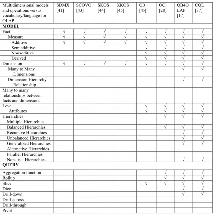
Table 3. The summary of the completeness of the linked cube data model and query

Multidimensional models and operations versus vocabulary/language for OLAP

SDMX [41]

SCOVO [43]

SKOS [44]

XKOS [45]

QB [46]

OC [28]

QB4O LAP [17]

CQL [37]

MODEL

Fact √ √ √ √ √ √ √ √

Measure √ √ √ √ √ √ √ √

Additive √ √ √ √ √ √ √ √

Semiadditive √ √ √ √

Nonadditive √ √ √ √

Derived √ √ √ √

Dimension √ √ √ √ √ √ √ √

Many to Many Dimensions

√ √

Dimension Hierarchy

Relationship √ √

Many to many relationships between facts and dimensions

Level √ √ √ √

Attributes √ √ √ √

Hierarchies √ √ √

Multiple Hierarchies

Balanced Hierarchies √ √ √

Recursive Hierarchies √ √

Unbalanced Hierarchies √ √

Generalized Hierarchies √ √

Alternative Hierarchies Parallel Hierarchies

Nonstrict Hierarchies √ √

QUERY

Aggregation function √ √ √

Rollup √ √ √

Slice √ √ √ √

Dice √ √

Drill-down √ √

Drill-across Drill-through Pivot

5 SPATIOTEMPORAL DATABASE

Spatiotemporal database is a database that stores information from spatiotemporal objects and manages the data for query retrieval. Every object has space and time attributes, these objects are called spatiotemporal objects. Along with GPS technology and location-based technology, the number of spatiotemporal objects and spatiotemporal data has increased in quantity. Spatiotemporal objects have spatial and temporal attributes and their combinations. Spatial attributes describe real-world phenomena consisting of descriptive components, which are presented with traditional

ISSN: 1992-8645 www.jatit.org E-ISSN: 1817-3195

3621

Table 4. Operator in spatial data types

Class Operators Topological

Operations (RCC8)

Intersects, Disjoint, Equal, Overlaps, Contains, Within, Touches, Covers, CoveredBy, Crosses

Predicates (Boolean) IsEmpty, OnBorder, InInterior Unary Operations Boundary, Buffer, Centroid,

ConvexHull

Binary Operations Intersection, Union, Difference, SymDifference

Numeric NoComponents, Length, Area, Perimeter, Distance,

HaversineDistance,Direction,NoOfInteri orRings

Spatial Aggregation Intersection, Union, ConvexHull, MinimumBoundingRectangle, Center of n Point, Center of Gravity,

Equipartition, Nearest-neighbor index Azimuthal

Relationship and Direction

North, South, East, West, Direction

Figure 7. Examples of spatial type operators [1]

Temporal attributes describe time, changing in time that the value could be represented by temporal types. For instance, temporal integers could be used to describe the evolution of employee salary, temporal geometries represent the area of an agricultural field that decreases every year, temporal points denote the flight path data from an aircraft and tourist movement from one place to another as reported as GPS device. The temporal type has subtype like boolean, integer, float, text, and geometric. Depending on the subtype, temporal types could be discrete or continuous. Discrete temporal types evolve in a stepwise manner like boolean, integer, and text, but continuous temporal types evolved in a continuous manner like float and geometric. The example of the temporal float is the temperature of the human body, on the other hand, the example of temporal geometric (point) is the location of a truck read by GPS device.

Temporal types are based on four-time types: timestamp with time zone, period, timestamp set,

and period set. A value of period type has two bounds, lower and upper with timestamp type. Temporal types recognize duration that states the temporal extent at which the evolution of values is recorded. The temporal type also distinguishes valid time and transaction time. Valid time is the time when the value of a tuple is valid in the database, while the transaction time is the time at which tuples are recorded in the database. For example, if the salary of an employee is recorded in the database on January 28, 2014, this will be stored as its transaction time, but if it holds for the employee from February 28, 2014, the later date will be recorded as the valid time for this attribute. Figure 3 illustrates an example of simple temporal attributes that represent salary changes. John’s salary is 20 that valid from January 1, 2012, until July 1, 2012, and 30 that valid from October 1, 2012, until January 1, 2013. On the other hand, Mary’s salary is 60 that valid from April 1, 2012, until April 1, 2013. 

Figure 8 Examples of salary change [1]

Temporal types have an associated set of operators, as shown in table 5.

Table 5. Operator in temporal types

Class Operators Projection to

domain/range

DefTime, RangeValues, Trajectory

Predicates

(Boolean) IsDefinedAt,isContinousIn Interaction with

domain/range GetValue, HasValue, AtInstant, AtPeriod,InitialInstant, InitialValue, FinalInstant, FinalValue,At, AtMin, AtMax, startSequence, endSequence, etc Unary

Operations(Spatial)

Length, Transform, CummulativeLength, NearestApproachDistance Binary Operations Before, Equals, Meets, Overlaps,

During, Start, Finish Rate of Change Derivative, Speed, Turn Temporal

Aggregation Integral, Duration, Length, TAvg, TVariance, TStDev, TMin, TMax Lifting All new operations inferred

5.1 Temporal Spatial Types

3622 This combination occurs in moving objects, such as moving pedestrians, moving trucks, moving clouds, shrinking agricultural areas. All operations for temporal types are also valid for spatial types. The following figure 9 is an example of moving trucks in a palm oil simulation plant. 

Figure 9. Examples of temporal-spatial types: moving trucks

The more details of the examples of moving objects are depicted in the following figure 10. Figure 10 displays the example of a moving pedestrian that can be manipulated using the temporal operator in table 4. Someone (f) walks from location A (0,2) at 8:00 to location B (8,9) and arrives at 08:10 proceed (g) to location E (12,9) and arrives at 08:15, and someone (h) walks from location D (1,1) at 8:00 to location E (12,5). The distance of the moving pedestrian is varying in time that depicted in figure 11.

Figure 10. Examples of moving pedestrians

Figure 11. The distance of the moving pedestrians 

The temporal-spatial types could be extended to represent field/region that varies both in time and space. The examples of this representation are the area that is shrinking every year at a certain speed. The illustration of the phenomena is depicted in

figure 11. The grey area is a missing area that becomes bigger every year.

Figure 12. Example of shrinking regions

The spatiotemporal database is then used to store spatial types, temporal types, and temporal-spatial types. This database could store the position of moving objects at any point in time, regions with the reduced area continuously, and so on. Although some examples of queries could be solved like “When did an airplane from Jakarta coded KL870 arrive at Kuala Lumpur International Airport?”, “How fast is the reduction of rainforests in Kalimantan in the last 5 years?”, but this kind of databases do not provide a foundation for complex analytical queries such as “How many total numbers of transports started in Kuala Lumpur in January, February, and March 2012?” or “How long average duration of transportations by region.” These kind of queries could be handled efficiently using DW, and the DW could be extended in order to support the concept of spatiotemporal data warehouses that contain spatial types, temporal types, and temporal-spatial types data.

0 1 2 3 4 5 6

1 2 3 4 5 6 7 8 9 10 11 12

distance

Time

year 2010

ISSN: 1992-8645 www.jatit.org E-ISSN: 1817-3195

3623

6 SPATIOTEMPORAL DATA

WAREHOUSE

Spatiotemporal DW is an infrastructure of OLAP that performs on spatial and temporal data. Spatiotemporal DW, which attracts researchers in the early 2000s, is a combination of GIS and OLAP that support spatial data types, temporal data types, temporal-spatial data types (moving object types) and evolving data warehouse dimensions. Exploration for a spatial data warehouse for the first time has been conducted by the design of spatial dimension hierarchy in the form of geometric and non-geometric attributes [50]. Rivest et al. began to study spatiotemporal DW by combining GIS and time with OLAP, with defining operators such as drill-down and roll-up on maps. This study succeeded in identifying features and operators imposed on spatiotemporal databases [51].

Furthermore, Da Silva et al. designed and built the GeoDWFrame framework, a framework of processing Geographical Data Warehouse and the GeoMDQL language used in the Spatial Cube based on geographical or hybrid dimension, MDX, and Open Geospatial Consortium (OGC) features [52]. Malinowsky et al. discovered the MultiDim conceptual model, which could model several spatial and temporal features, like spatial dimension, and spatial level using topological relationship. In the MultiDim model, the spatial measure could be represented by geometry, which is an aggregation of dimensions, or aggregation of numerical value representing in shape which is calculated based on topology operators and metric operators. Almost all proposals for geometry aggregation are represented in sets of coordinates or sets of pointers to objects [53]. The spatial extension of the MultiDim model based on the spatial data types of MADS also found in [54]. A great discovery of the integration of GIS and OLAP arises when Gomez et al. found geometric data aggregation, and measure associated with component aggregation. In this research, a combination of GIS and OLAP is maintained through a language, GISOLAP-QL. They also developed a framework called Piet, which provides four features of queries, including the standard query of GIS, OLAP, geometric aggregation, and integrated GIS-OLAP queries. The examples of geometric aggregation are like “how many total population in the district through which more than three river pass”, and the examples of integrated

GIS-OLAP query is like “how many average crop production by-product by district around the slopes of the mountain”. Furthermore, Piet outfits a new query processing using decomposition technique to split the thematic layer in a GIS, into open convex polygons; then, implement the overlay precomputation as a materialization technique [55].

Moreover, modeling and querying

spatiotemporal data has been demonstrated by the framework SECONDO. SECONDO was developed as a DBMS platform that can implement several data models, such as Spatio-temporal data, and graph models, and run a query on these data models [56], [57]. SECONDO has been extended to Distributed SECONDO as a scalable and fault-tolerant DBMS using Apache Cassandra as data storage [58]. Additionally, HERMES, a robust framework capable of modeling, constructing and querying spatiotemporal databases that are implemented in the Relational DBMS Object [59]. Spatiotemporal databases are then developed into spatiotemporal DW, which put forward the concept of a trajectory DW that provides an infrastructure for aggregating mobile data objects and mining data. This study also puts forward an efficient ETL process from track observation data to DW [60]. Braz et al. introduce the term of Trajectory DW by extending the conventional DW to store trajectory aggregation of the moving objects, and implement the OLAP operations over the trajectory DW. Trajectory DW is able to analyze interesting measures of mobility objects such as the number, speed, and acceleration of moving objects in a particular region and other measures [61]. The Trajectory DW makes trajectory data become valuable knowledge, which provides a basic foundation for a wide range of applications such as traffic management and control, analysis of social behavior, and recommender system [62]. Trajectory DW has been successfully implemented in PostGIS, an extended version of PostgreSQL with OGC based model [63]. Trajectory DW also could be used to organize and analyze trajectory data using OLAP and data mining techniques [64].

3624 in the form of long sequences of spatiotemporal coordinates (x, y, t), and store the positions of moving objects at any point in time. This DW contains mobility object data that can be analyzed in combination with other kinds of data (e.g., spatial data), for instance, a road network, altitude data, and the kind [67].

On the other hand, in the absence of a commonly agreed definition of what is a Spatio-temporal DW and what functionality it should support. Vaisman and Zimanyi present a conceptual framework for defining spatiotemporal DW using an extensible datatype system. This conceptual framework defines a taxonomy of models that integrate OLAP, spatial data, and moving data types. From the classes in this taxonomy, they also represent queries from tuple relational calculus, extended aggregate functions to spatiotemporal calculus supporting moving data types [68]. Spatiotemporal DW taxonomy is categorized into four classes, namely: Temporal dimensions, OLAP, GIS, and moving data types. The combination of these classes is shown in the following picture:

Figure 13. Taxonomy of Spatiotemporal OLAP [1]

Combining GIS with Moving Data Types produces Spatiotemporal data, OLAP, and GIS resulting in SOLAP, OLAP and Spatiotemporal Data resulting in Spatiotemporal OLAP, Temporal Dimension and Spatiotemporal OLAP resulting in Spatiotemporal TOLAP. Temporal Dimensions and OLAP produce TOLAP, while TOLAP combined with GIS becomes Spatial TOLAP. The taxonomy also produces different queries for each class. Examples of queries from each taxonomy are as follows:

1. OLAP: For each field in a particular village and certain districts show the total production of three types of plants: rice, corn, and soybeans, every year.

2. Spatial OLAP: Show the total production of three types of plants: rice, corn and soybeans, each year at a distance of 10 km from the peak of Mount X in Central Java Indonesia.

3. Temporal OLAP: For each village and type of plant, show average production in the first quartile of 2018, for each location of water pollution monitoring, give information on how many days in a year where pollution levels exceed the threshold.

4. Spatiotemporal OLAP (ST-OLAP): For certain types of plants at a radius of 10 km from the summit of Mount X how much is the total loss of harvest failure due to eruption in February 2019.

5. Spatio-Temporal OLAP (S-TOLAP): For each village above the Y river determine how long (in days) successive hot clouds hit

6. Spatiotemporal-Temporal OLAP (ST-TOLAP): What is the total number of days in which Z Regency is under at least one CO-charged cloud so that the average load of the cloud is greater than the load limit when the cloud appears

6.1 Conceptual Model Spatiotemporal Data

Warehouse

ISSN: 1992-8645 www.jatit.org E-ISSN: 1817-3195

3625 either numerical data or spatial data (geometry). The data measure type determines what operations can be imposed on it, by default sum is an operation for numerical measure and spatial union to measure geometry. Some types of spatial aggregation for a spatial type are distributive spatial (spatial union, spatial intersection, convex hull), spatial algebraic (center of n point, the center of gravity), spatial holistic (equipartition, nearest-neighbor index).

The examples of the DW that support spatiotemporal analysis is depicted in figure 14. The idea is developing spatiotemporal DW that keeps track of deliveries of fruit bunch in the plantation and analysis of fruit load/unloading from fruit collection points. In the company, there is an armada of trucks that load some fruits from several fruit collection points and transporting them into the loading ramp of the plant and unloading them for processing. The driver of the trucks performs a delivery according to an order from the plant. There are spatial data about the road network, the geographic hierarchy from the plantation (afdeling, block, and fruit collection point/FCP), and the trajectory traced by the trucks. Additionally, there are non-spatial data about drivers and the trucks. Figure 6 depicts the conceptual schema showing the scenario using MultiDim model extended to support spatial, temporal, and temporal-spatial types.

As shown in the figure, the fact Delivery is a spatial fact that related to five dimensions: Truck, Time, Plant, TruckDriver, and FruitCollectionPoint (FCP), where the latter is a spatial dimension related to the fact through a many-to-many relationship. The truck dimension is composed of two levels, with one-to-many relationships. Spatial attributes or levels have an associated geometry (e.g., point, line, and region), which is indicated by , and . In this example, dimensions Plant and FCP are spatial and share geography hierarchy where geometry is associated with each level in both dimensions. The FCP Dimension has a topological constraint that indicates an FCP is contained in Plantation Block and Plantation Block is contained in Plantation Afdeling and creates a parent-child relationship.

The spatial fact table Delivery has seven measures. The first measure is Route that captures the truck position at any point in time. This measure is a spatiotemporal measure of temporal point type, as shown by the symbol t(•). The other measures are derived from Route, measure Trajectory captures the

geometry of the route traversed by the truck, which is represented by a line, without temporal information, measure Distance, Load, and Duration are numeric, while StartTime and EndTime are timestamps. Trajectory measure is a spatial measure of line type, as shown by the symbol .

The Route measure as a temporal point type allowing Deliveries to be aggregated along the dimensions, for example the similar route could be merge into a single owner, the route could be union, intersect, etc. Thus, the query like “give 

me the total number trajectory by TruckOwner”, or

Figure 14. An example of the conceptual schema of the

spatiotemporal Data Warehouse

3626 Thus, Spatiotemporal Slice also possible to determine like query “Give the aggregate of fruit weight deliveries within the location of Block Geo (polygon (102.251223 55.4745345; 102.251233 55.474535;….)) in a week that begin from 28 March 2019”, spatiotemporal dice query like “Give the average duration of fruit deliveries from the FCD location and PlantGeo within 5 km in an hour interval from 7.00 AM on 28 March 2019, temporal aggregation query like “For truck with the velocity 20 km/h, give the total distance travelled by each of the truck”, and spatial slice like “Compute the deliveries that traversed at least two plantation afdeling”.

6.2 Spatiotemporal Multidimensional Data

Model on the Semantic Web

The semantic web continues to grow with various types of data, including for spatiotemporal data. Spatiotemporal data continues to grow due to the use of mobile devices, GPS, IoT, network sensors and location-based applications. Development of Spatiotemporal Multidimensional Data model on the semantic web starts from the Spatial Semantic Web, or commonly referred to as Geospatial Semantic Web. The Geospatial Semantic Web development began with the finding of a new retrieval method for geospatial data built on the semantics of spatial and ontologies developed at the University of Maine [69]. Then, Basic Geo Vocabulary has been standardized by W3C Semantic Web Interest Group using WGS84 as a reference datum [70].

Perry et al. instated that the Web has abundant spatial and temporal data, and the technology of SW potentially could make the accessibility and usefulness of data better. Because of the lack of ability of SPARQL to query complex spatial and temporal data, therefore Perry et al. proposed a new query language SPARQL- ST, which an extension of SPARQL for complex spatiotemporal queries. This research suggested a formal syntax and semantics and also added spatial variables and constructs for manipulating temporal triples in SPARQL-ST and applied as a prototype built on top of a commercial DBMS [71]. This is the approach that combines spatiotemporal semantic web, but limited only for basic operation for spatiotemporal like a topological and temporal relationship, but not for aggregation and analytic query functions.

Research continues to grow and has been successfully implemented such as Linked Geospatial Data in the UK government, followed by the manufacture of geospatial datasets by the Ordnance Survey Company for regions in the UK that can be accessed using SPARQL Endpoints [72]. Linked data becoming popular with the advent of Geonames, which is a dataset in the form of linked data that collects spatial and thematic information for place names in various hemispheres in various languages. The information stored in it is in the form of latitude, longitude, altitude, population, and administrative information with the rules of the World Geodetic System 1984 (WGS84). Furthermore, there is LinkedGeodata, which is a linked data which is a semantic web infrastructure that is converted from OpenStreetMap, this linked data is very useful for integrating and aggregating data related to maps [73] and can be easily queried with SPARQL. This approach attracts many researchers as a promising spatial linked data paradigm, but still, this approach did not cover temporal data.

The temporal aspect then entered as a Spatiotemporal Semantic Web on the development of YAGO2 ontology which is a continuation of YAGO knowledge-based ontology where entities, events, and facts are combined with information on space and time. YAGO2 was developed by automating Wikipedia, GeoNames, and WordNet linked data. At present YAGO2 contains 447 million facts and 9.8 million entities. YAGO2 uses the SPOTL model data (5 tuples), which is the extension of SPO (3 tuples). Entities on YAGO2 are assigned a time span, while fact is assigned a time point or time span [74]. YAGO2 become a good methodology for enriching large spatiotemporal knowledge bases but this approach did not have a query extension for this spatiotemporal representation.

ISSN: 1992-8645 www.jatit.org E-ISSN: 1817-3195

3627 of the GeoSPARQL is built to be small for easily understood and attached. GeoSPARQL ontology has two main classes: Feature and Geometry. A Feature is an entity with spatial attributes. An example of the Feature is a building, statue, palace, lake, etc. A Geometry is a shape, for example, a point, line, triangle, hexagon, etc. and is used as a representation of a feature’s spatial location. The third class, SpatialObject, is a superclass of both Feature and Geometry. GeoSPARQL has become as a geospatial RDF standard from W3C for data modeling and querying [76]. GeoSPARQL has some impressive features for geospatial implementation on SW, but this language did not accommodate for analytical query dan has no extension for spatiotemporal and mobility data representation and query.

Further, EU research running the GeoKnow project for three years from late 2012 to 2015. This project is the extension of the LinkedGeoData project, which develops OpenStreetMap that makes data available as an RDF base. The project applies the RDF model and the GeoSPARQL standard as the basis for representing and querying geospatial data. GeoKnow contributive findings are (a) introduction of query optimization methods of geospatial RDF for better performance than existing RDF store, even still lack analysis performances compared to relational DBMS (b) aggregation of geospatial RDF data with fusion [77]. The adoption of the RDF Triple store for Semantic Geospatial and GeoSPARQL queries developed with the advent of Parliament RDF [78].

Another proposal similar to GeoSPARQL is the development of stRDF/stSPARQL. The stRDF is a data model with an extension of RDF to represent geospatial information that changes over time [79]. stRDF defines spatial and temporal dimensions that have literal spatial and spatial data types. stRDF also uses OGC standards like WKT and GML for serialization. stSPARQL was developed as an extension query language for SPARQL by adding function defined in the OpenGIS standard Simple Feature Access. These functions are in the form of basic functions (get, test), basic function access functions (equals, disjoint, intersect, touches, crosses, within, contains, overlaps, relate), Egenhofer, RCC8, spatial analysis functions, spatial metric functions (distance, area), the function of aggregate spatial (union, intersection, extent). Strabon was then developed as an RDF store that

supports semantic geospatial query languages in stSPARQL and GeoSPARQL. Strabon has expressive power by these query languages with the data stRDF model. The Performance of Strategic scales to vast volumes of data and performs well [79]. stRDF/stSPARQL has accommodated many features of spatial data representation and query implementations, but it still lacks spatiotemporal data adoption and analytical capabilities.

Zhang et al. proposed an extension of SPARQL to spatiotemporal modeling and querying a quantitative spatiotemporal relationship. The extension model is adding an event model with time and space. The query extension created 30 new query operators that claimed could effectively find the unseen connections between entities in event ontology and have excellent performance and effectiveness [80]. This approach comprehensively adds the functionality of SPARQL but this approach still does not handle the spatiotemporal analytical query.

On the other hand, Gur et al. proposed QB4SOLAP, a generic and extensible vocabulary (meta-model) for spatial DW on the SW. QB4SOLAP extends QB4OLAP vocabulary with spatial concepts. They also give a formalization of QB4SOLAP. This paper has defined the critical concepts of spatial cube numbers, spatial hierarchies and levels, spatial measures, spatial aggregation functions, and topological relations among spatial dimension and hierarchy level members. They also defined several analytical spatial OLAP operators over QB4SOLAP, the formal semantics of these operators, and algorithms for generating spatially extended SPARQL queries [8]. This work has a significant result for modeling and querying spatial analytical data but this work is only limited for spatial data and not for spatiotemporal data that have the more dynamic characteristics.