Image Mosaicing for Tele-Reality
Applications
Richard Szeliski
Digital Equipment Corporation Cambridge Research Lab
Digital Equipment Corporation has four research facilities: the Systems Research Center and the Western Research Laboratory, both in Palo Alto, California; the Paris Research Laboratory, in Paris; and the Cambridge Research Laboratory, in Cambridge, Massachusetts.
The Cambridge laboratory became operational in 1988 and is located at One Kendall Square, near MIT. CRL engages in computing research to extend the state of the computing art in areas likely to be important to Digital and its customers in future years. CRL’s main focus is applications technology; that is, the creation of knowledge and tools useful for the preparation of important classes of applications.
CRL Technical Reports can be ordered by electronic mail. To receive instructions, send a mes-sage to one of the following addresses, with the word help in the Subject line:
On Digital’s EASYnet: CRL::TECHREPORTS On the Internet: [email protected]
This work may not be copied or reproduced for any commercial purpose. Permission to copy without payment is granted for non-profit educational and research purposes provided all such copies include a notice that such copy-ing is by permission of the Cambridge Research Lab of Digital Equipment Corporation, an acknowledgment of the authors to the work, and all applicable portions of the copyright notice.
The Digital logo is a trademark of Digital Equipment Corporation.
Cambridge Research Laboratory One Kendall Square
Cambridge, Massachusetts 02139
Image Mosaicing for Tele-Reality
Applications
Richard Szeliski
Digital Equipment Corporation Cambridge Research Lab
CRL 94/2 May, 1994
Abstract
While a large number of virtual reality applications, such as fluid flow analysis and molecular modeling, deal with simulated data, many newer applications attempt to recreate true reality as convincingly as possible. Building detailed models for such applications, which we call tele-reality, is a major bottleneck holding back their deployment. In this paper, we present techniques for automatically deriving realistic 2-D scenes and 3-D texture-mapped models from video sequences, which can help overcome this bottleneck. The fundamental technique we use is image mosaicing, i.e., the automatic alignment of multiple images into larger aggregates which are then used to represent portions of a 3-D scene. We begin with the easiest problems, those of flat scene and panoramic scene mosaicing, and progress to more complicated scenes, culminating in full 3-D models. We also present a number of novel applications based on tele-reality technology.
Keywords: image mosaics, image registration, image compositing, planar scenes, panoramic scenes, 3-D scene recovery, motion estimation, structure from motion, virtual reality, tele-reality.
Contents i
Contents
1 Introduction
: : : : : : : : : : : : : : : : : : : : : : : : : : : : : : : : : : : : : : :
1 2 Related work: : : : : : : : : : : : : : : : : : : : : : : : : : : : : : : : : : : : : :
2 3 Basic imaging equations: : : : : : : : : : : : : : : : : : : : : : : : : : : : : : : :
3 4 Planar image mosaicing: : : : : : : : : : : : : : : : : : : : : : : : : : : : : : : :
54.1 Local image registration
: : : : : : : : : : : : : : : : : : : : : : : : : : : : : :
6 4.2 Global image registration: : : : : : : : : : : : : : : : : : : : : : : : : : : : :
8 4.3 Results: : : : : : : : : : : : : : : : : : : : : : : : : : : : : : : : : : : : : : :
85 Panoramic image mosaicing
: : : : : : : : : : : : : : : : : : : : : : : : : : : : : :
95.1 Results
: : : : : : : : : : : : : : : : : : : : : : : : : : : : : : : : : : : : : : :
116 Scenes with arbitrary depth
: : : : : : : : : : : : : : : : : : : : : : : : : : : : : :
116.1 Formulation
: : : : : : : : : : : : : : : : : : : : : : : : : : : : : : : : : : : :
13 6.2 Results: : : : : : : : : : : : : : : : : : : : : : : : : : : : : : : : : : : : : : :
147 Full 3-D model recovery
: : : : : : : : : : : : : : : : : : : : : : : : : : : : : : : :
14 8 Applications: : : : : : : : : : : : : : : : : : : : : : : : : : : : : : : : : : : : : : :
188.1 Planar mosaicing applications
: : : : : : : : : : : : : : : : : : : : : : : : : : :
18 8.2 3-D model building applications: : : : : : : : : : : : : : : : : : : : : : : : : :
19 8.3 End-user applications: : : : : : : : : : : : : : : : : : : : : : : : : : : : : : :
19ii LIST OF FIGURES
List of Figures
1 Introduction 1
1
Introduction
Virtual reality is currently creating a lot of excitement and interest in the computer graphics community. Typical virtual reality systems use immersive technologies such as head-mounted or stereo displays and data gloves. The intent is to convince users that they are interacting with an alternate physical world, and also often to give insight into computer simulations, e.g., for fluid flow analysis or molecular modeling [Earnshaw et al., 1993]. Realism and speed of rendering are therefore important issues.
Another class of virtual reality applications attempts to recreate true reality as convincingly as possible. Examples of such applications include flight simulators (which were among the earliest uses of virtual reality), various interactive multi-player games, and medical simulators, and visualization tools. Since the reality being recreated is usually distant, we use the term
tele-reality in this paper to refer to such virtual tele-reality scenarios based on real imagery.1 Tele-reality applications which could be built using the techniques described in this paper include scanning a whiteboard in your office to obtain a high-resolution image, walkthroughs of existing buildings for re-modeling or selling, participating in a virtual classroom, and browsing through your local supermarket aisles from home (see Section 8.)
While most focus in virtual reality today is on input/output devices and the quality and speed of rendering, perhaps the biggest bottleneck standing in the way of widespread tele-reality applications is the slow and tedious model-building process [Adam, 1993]. This also affects many other areas of computer graphics, such as computer animation, special effects, and CAD. For small objects, say 0.2–2m, laser-based scanners are a good solution. These scanners provide registered depth and colored texture maps, usually in either raster or cylindrical coordinates [Cyberware Laboratory Inc, 1990; Rioux and Bird, 1993]. They have been used extensively in the entertainment industry for special effects and computer animation. Unfortunately, laser-based scanners are fairly expensive, limited in resolution (typically 512256 pixels), and most importantly, limited in range (e.g., they
cannot be used to scan in a building.)
The image-based ranging techniques which we develop in this paper have the potential to overcome these limitations. Imagine walking through an environment such as a building interior and filming a video sequence of what you see. By registering and compositing the images in the
1
The term telepresence is also often used, especially for applications such as tele-medicine where two-way
2 2 Related work
video together into large mosaics of the scene, image-based ranging can achieve an essentially unlimited resolution.2 Since the images can be acquired using any optical technology (from
microscopy, through hand-held videocams, to satellite photography), the range or scale of the scene being reconstructed is not an issue. Finally, as desktop video becomes ubiquitous in our computing environments—initially for videoconferencing, and later as an advanced user interface tool [Gold, 1993; Rehg and Kanade, 1994; Blake and Isard, 1994]—image-based scene and model acquisition will become accessible to all users.
In this paper, we develop novel techniques for extracting large 2-D textures and 3-D models from image sequences based on image registration and compositing techniques and also present some potential applications. After a review of related work (Section 2) and of the basic image formation equations (Section 3), we present our technique for registering pieces of a flat (planar) scene, which is the simplest interesting image mosaicing problem (Section 4). We then show how the same technique can be used to mosaic panoramic scenes obtained by rotating the camera around its center of projection (Section 5). Section 6 discusses how to recover depth in scenes. Section 7 discusses the most general and difficult problem, that of building full 3-D models from multiple images. Section 8 presents some novel applications of the tele-reality technology developed in this paper. Finally, we close with a comparison of our work with previous approaches, and a discussion of the significance of our results.
2
Related work
While 3-D models acquired with laser-based scanners are now commonly used in computer ani-mations and for special effects, 3-D models derived directly from still or video images are still a rarity. One example of physically-based models derived from images are the dancing vegetables in the “Cooking with Kurt” video [Terzopoulos and Witkin, 1988]. Another, more recent example, is the 3-D model of a building extracted from a video sequences in [Azarbayejani et al., 1993], which was then composited with a 3-D teapot. Somewhat related are graphics techniques which extract camera position information from images, such as [Gleicher and Witkin, 1992].
2
The traditional use of the term image compositing [Porter and Duff, 1984; Foley et al., 1990] is for blending
images which are already registered. We use the term image mosaicing in this paper for our work to avoid confusion
3 Basic imaging equations 3
The extraction of geometric information from multiple images has long been one of the central problems in computer vision [Ballard and Brown, 1982; Horn, 1986] and photogrammetry [Moffitt and Mikhail, 1980]. However, many of the techniques used are based on feature extraction, produce sparse descriptions of shape, and often require manual assistance. Certain techniques, such as stereo, produce depth or elevation maps which are inadequate to model true 3-D objects. In computer vision, the recovered geometry is normally used either for object recognition or for grasping and navigation (robotics). Relatively little attention has been paid to building 3-D models registered with intensity (texture maps), which are necessary for computer graphics and virtual reality applications (but see [Mann, 1993] for recent work which addresses some of the same problems as this paper.)
In computer graphics, compositing multiple image streams together to create larger format (Omnimax) images is discussed in [Greene and Heckbert, 1986]. However, in this application, the relative position of the cameras was known in advance. The registration techniques developed in this paper are related to image warping [Wolberg, 1990] since once the images are registered, they can be warped into a common reference frame before being composited.3 While most current
techniques require the manual specification of feature correspondences, some recent techniques [Beymer et al., 1993] as well as the techniques developed in this paper can be used to automate this process. Combinations of local image warping and compositing are now commonly used for special effects under the general rubric of morphing [Beier and Neely, 1992]. Recently, morphing based on z-buffer depths and camera motion has been applied to view interpolation as a quick alternative to full 3-D rendering [Chen and Williams, 1993]. The techniques we develop in Section 6 can be used to compute the depth maps necessary for this approach directly from real-world image sequences.
3
Basic imaging equations
Many of the ideas in this paper have their simplest expression using projective geometry [Semple and Kneebone, 1952]. However, rather than relying on these results, we will use more standard methods and notations from computer graphics [Foley et al., 1990], and prove whatever simple
3
One can view the image registration task as an inverse warping problem, since we are given two images and asked
4 3 Basic imaging equations
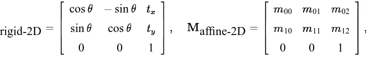
Figure 1: Rigid, affine, and projective transformations
results we require in Appendix A. Throughout, we will use homogeneous coordinates to represent points, i.e., we denote 2-D points in the image plane as (
xyw
), with (x=wy=w
) being thecorresponding Cartesian coordinates [Foley et al., 1990]. Similarly, 3-D points with homogeneous coordinates(
xyzw
)have Cartesian coordinates(x=wy=wz=w
).Using homogeneous coordinates, we can describe the class of 2-D planar transformations using matrix multiplication 2 6 6 6 4
x
0y
0w
0 3 7 7 7 5 = 2 6 6 6 4m
00m
01m
02m
10m
11m
12m
20m
21m
22 3 7 7 7 5 2 6 6 6 4x
y
w
3 7 7 7 5or
u
0=
M
2Du
:
(1)The simplest transformations in this general class are pure translations, followed by translations and rotations (rigid transforms), plus scaling (similarity transforms), affine transforms, and full projec-tive transforms. Figure 1 shows a square and possible rigid, affine, and projecprojec-tive transformations. Rigid and affine transformations have the following forms for the
M
2Dmatrix,M
rigid-2D= 2 6 6 6 4cos
;sint
xsin
cost
y0 0 1
3 7 7 7
5
M
affine-2D = 2 6 6 6 4m
00m
01m
02m
10m
11m
120 0 1
3 7 7 7 5
with 3 and 6 degrees of freedom, respectively, while projective transformations have a general
M
2Dmatrix with 8 degrees of freedom.4
In 3-D, we have the same hierarchy of transformations, with rigid (6 degrees of freedom), similarity (7 dof), affine (12 dof), and full projective (15 dof) transforms. The
M
3Dmatrices in this4
Two
M
2Dmatrices are equivalent if they are scalar multiples of each other. We remove this redundancy by setting4 Planar image mosaicing 5
case are 44. Of particular interest are the rigid (Euclidean) transformation,
E
= 24
R t
0
T1
3
5
(2)where
R
is a 33 orthonormal rotation matrix andt
is a 3-D translation vector, and the 34viewing matrix
V
= hˆ
V 0
i = 2 6 6 6 41 0 0 0
0 1 0 0
0 0 1
=f
03 7 7 7 5
(3)which projects 3-D points through the origin onto a 2-D projection plane a distance
f
along thez
axis [Foley et al., 1990]. The 33 ˆV
matrix can be a general matrix in the case where the internalcamera parameters are unknown. The last column of
V
is always zero for central projection. The combined equations projecting a 3-D world coordinatep
=(xyzw
)onto a 2-D screenlocation
u
=(x
0y
0w
0)can thus be written as
u
=VEp
=M
camp
(4)where
M
cam is a 3 4 camera matrix. This equation is valid even if the camera calibrationparameters and/or the camera orientation are unknown.
4
Planar image mosaicing
The simplest possible set of images to mosaic are pieces of a planar scene such as a document, whiteboard, or flat desktop. Imagine that we have a camera fixed directly over our desk. As we slide a document under the camera, different portions of the document are visible. Any two such pieces are related to each other by a translation and a rotation (2-D rigid transformation).
6 4 Planar image mosaicing
Given this knowledge, how do we go about computing the transformations relating the various scene pieces so that we can paste them together? A variety of techniques are possible, some more automated than others. For example, we could manually identify four or more corresponding points between the two views, which is enough information to solve for the eight unknowns in the 2-D projective transformation. Or we could iteratively adjust the relative positions of input images using either a blink comparator or transparency [Carlbom et al., 1991]. These kinds of manual approaches are too tedious to be useful for large tele-reality applications.
4.1
Local image registration
The approach we use in this paper is to directly minimize the discrepancy in intensities between pairs of images after applying the transformation we are recovering. This has the advantage of not requiring any easily identifiable feature points, and of being statistically optimal once we are in the vicinity of the true solution [Szeliski and Coughlan, 1994]. More concretely, suppose we describe our 2-D transformations as
x
0 i=
m
0x
i+
m
1y
i+
m
2m
6x
i+
m
7y
i+ 1
y
0 i=
m
3x
i+
m
4y
i+
m
5m
6x
i+
m
7y
i+ 1
:
(5)Our technique minimizes the sum of the squared intensity errors
E
= X iI
0 (x
0 iy
0 i);
I
(x
iy
i)] 2 = X i
e
2 i (6)over all corresponding pairs of pixels
i
which are inside both imagesI
(xy
)andI
0(
x
0y
0)(pixels
which are mapped outside image boundaries do not contribute.) Once we have found the best transformation
M
2D, we can warp imageI
0
into the reference frame of
I
usingM
;12D [Wolberg,
1990] and then blend the two images together. To reduce visible artifacts, we weight images being blended together more heavily towards the center, using a bilinear weighting function.
To perform the minimization, we use the Levenberg-Marquardt iterative non-linear minimiza-tion algorithm [Press et al., 1992]. This algorithm requires the computaminimiza-tion of the partial derivatives of
e
i with respect to the unknown motion parametersf
m
0:::m
7g. These are straightforward tocompute, i.e.,
@e
i@m
0 =x
iD
i@I
04.1 Local image registration 7
where
D
i is the denominator in (5), and (@I
0
=@x
0@I
0=@y
0)is the image intensity gradient of
I
0at (
x
0 iy
0 i
). From these partials, the Levenberg-Marquardt algorithm computes an approximate
Hessian matrix
A
and the weighted gradient vectorb
with componentsa
k l = X i@e
i@m
k@e
i@m
lb
k =;2X i
e
i@e
i@m
k (8)and then updates the motion parameter estimate
m
by an amount∆m
= (A
+I
) ;1b
, where
is a time-varying stabilization parameter [Press et al., 1992]. The advantage of using Levenberg-Marquardt over straightforward gradient descent is that it converges in fewer iterations. The complete registration algorithm thus consists of the following steps:1. For each pixel
i
at location(x
iy
i),
(a) compute its corresponding position in the other image(
x
0 iy
0 i
)using (5);
(b) compute the error in intensity between the corresponding pixels
e
i =I
0 (x
0 iy
0 i);
I
(x
iy
i)
and the intensity gradient(
@I
0
=@x
0@I
0=@y
0 );(c) compute the partial derivative of
e
iw.r.t. them
k using@e
i@m
k =@I
0@x
0@x
0@m
k +@I
0@y
0@y
0@m
kas in (7);
(d) add the pixel’s contribution to
A
andb
as in (8).2. Solve the system of equations(
A
+I
)∆m
=b
and update the motion estimatem
(t+1)=
m
(t)+∆
m
.3. Check that the error in (6) has decreased; if not, increment
(as described in [Press et al., 1992]) and compute a new∆m
,4. Continue iterating until the error is below a threshold or a fixed number of steps has been completed.
8 4 Planar image mosaicing
4.2
Global image registration
Unfortunately, both gradient descent and Levenberg-Marquardt only find locally optimal solutions. If the motion between successive frames is large, we must use a different strategy to find the best registration. We have implemented two different techniques for dealing with this problem. The first technique, which is commonly used in computer vision, is hierarchical matching, which first registers smaller, subsampled versions of the images where the apparent motion is smaller [Quam, 1984; Witkin et al., 1987; Bergen et al., 1992]. Motion estimates from these smaller coarser levels are then used to initialize motion estimates at finer levels, thereby avoiding the local minimum problem (see [Szeliski and Coughlan, 1994] for details.) While this technique is not guaranteed to find the correct registration, we have observed empirically that it works well when the initial misregistration is only a few pixels (the exact domain of convergence depends on the intensity pattern in the image.)
For larger displacements, we use phase correlation [Kuglin and Hines, 1975; Brown, 1992]. This technique estimates the 2-D translation between a pair of images by taking 2-D Fourier Transforms of each image, computing the phase difference at each frequency, performing an inverse Fourier Transform, and searching for a peak in the magnitude image. In our experiments, this technique has proven to work remarkably well, providing good initial guesses for image pairs which overlap by as little as 50%. The technique will not work, however, if the inter-frame motion is not mostly translational (large rotations or zooms), but this does not occur in practice with our current image sequences.
4.3
Results
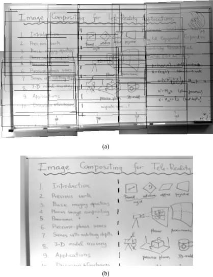
To demonstrate the performance of our algorithm, we digitized an image sequence with a camera panning over a whiteboard. Figure 2a shows the final mosaic of the whiteboard, with the locations of the constituent images in the mosaic shown as black outlines. Figure 2b is a portion of the final mosaic without these outlines. This mosaic is 13002046 pixels, based on compositing 39 NTSC
(640480) resolution images.
5 Panoramic image mosaicing 9
using phase correlation. Our algorithm then refines the location of each image by minimizing (6) using the current mosaic thus far as
I
(xy
)and the input frame being adjusted asI
0 (
x
0
y
0 ). Theimages in Figure 2 were automatically composited without user intervention using the middle frame (center of the image) as the anchor image (no deformations.) As we can see, our technique works well on this example. Section 9 discusses some imaging artifacts which can cause difficulties.
5
Panoramic image mosaicing
Another image mosaicing problem which turns out to be equally simple to solve is panoramic image mosaicing. In this scenario, we rotate a camera around its optical center in order to create a full “viewing sphere” of images (in computer graphics, this representation is sometimes called an environment map [Greene, 1986].) This is similar to the action of panoramic still photographic cameras where the rotation of a camera on top of a tripod is mechanically coordinated with the film transport, the anamorphic lens used in [Lippman, 1980], and to “cinema in the round” movie theaters [Greene and Heckbert, 1986]. In our case, however, we can mosaic multiple 2-D images of arbitrary detail and resolution, and we need not know the camera motion. Examples of applications include constructing true scenic panoramas (say of the view at the rim of the Grand Canyon), or limited virtual environments (recreating a meeting room or office as seen from one location.)
It turns out that images taken from the same viewpoint (stationary optical center) are related by 2-D projective transformations, just as in the planar scene case (see Appendix A for a quick proof.) Intuitively, we cannot tell the relative depth of points in the scene as we rotate (there is no
motion parallax), so they may as well be located on any plane (in projective geometry, we could
say they lie on the plane at infinity,
w
=0.) For some applications, this property is usually viewedas a deficiency, i.e., we cannot recover scene depth from rotational camera motion. For image mosaicing, this is actually an advantage since we just want to composite a large scene and be able to “look around” from a static viewpoint.
More formally, the 2-D transformation denoted by
M
2D is related to the viewing matrices ˆV
and ˆ
V
0and the inter-view rotation
R
byM
2D =ˆ
V
0R
V
ˆ;1(9)
10 5 Panoramic image mosaicing
(a)
[image:16.612.97.515.93.636.2](b)
Figure 2: Whiteboard image mosaic example
5.1 Results 11
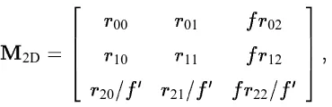
particularly simple form,
M
2D= 2 6 6 6 4r
00r
01fr
02r
10r
11fr
12r
20=f
0r
21
=f
0fr
22
=f
03 7 7 7 5
(10)
where
f
andf
0are the scaled focal lengths in the two views, and
r
k lare the entries in the rotationmatrix
R
.5 In this case, we only have to recover five independent parameters (or three if thef
values are known) instead of the usual eight.
How do we represent a panoramic scene composited using our techniques? One approach is to divide the viewing sphere into several large, potentially overlapping regions, and to represent each region with a plane onto which we paste the images [Greene, 1986]. Another approach is to compute the relative position of each frame relative to some base frame, and to then re-compute an arbitrary view on the fly from all visible pieces, given a particular view direction
R
and zoom factorf
. In our current implementation, we adopt the former strategy since it is a simple extension of the planar case. [image:17.612.215.400.119.179.2]5.1
Results
Figure 3 shows a mosaic of a bookshelf and cluttered desk, which is obviously a non-planar scene. The images were obtained by tilting and panning a video camera mounted on a tripod, without any special steps taken to ensure that the rotation was around the true center of projection. The complete scene is registered quite well.
6
Scenes with arbitrary depth
Mosaicing flat scenes or panoramic scenes may be interesting for certain tele-reality applications, e.g., transmitting whiteboard or document contents, or viewing an outdoor panorama. However, for most applications, we must recover the depth associated with the scene to give the illusion of a 3-D environment, e.g., through nearby view synthesis [Chen and Williams, 1993]. Two possible approaches are to model the scene as piecewise-planar or to recover dense 3-D depth maps.
5At large focal lengths and small rotations, M
12 6 Scenes with arbitrary depth
(a)
[image:18.612.156.459.103.622.2](c)
Figure 3: Panoramic image mosaic example (bookshelf and cluttered desk)
6.1 Formulation 13
The first approach is to assume that the scene is piecewise-planar, as is the case with many man-made environments such as building exteriors and office interiors. The image mosaicing technique developed in Section 4 can then be applied to each of the planar regions in the image. The segmentation of each image into its planar components can either be done interactively (e.g., by drawing the polygonal outline of each region to be registered), or automatically by associating each pixel with one of several global motion hypotheses [Jepson and Black, 1993; Wang and Adelson, 1993]. Once the independent planar pieces have been composited, we could, in principle, recover the relative geometry of the various planes and the camera motion (see Appendix A.) However, rather than pursuing this approach in this paper, we will purse the second, more general solution which is to recover a full depth map, i.e., to infer the missing
z
component associated with each pixel in a given image sequence.When the camera motion is known, the problem of depth map recovery is called stereo
recon-struction (or multi-frame stereo if more than two views are used [Matthies et al., 1989; Okutomi
and Kanade, 1993].) This problem has been extensively studied in photogrammetry and computer vision [Moffitt and Mikhail, 1980; Barnard and Fischler, 1982; Horn, 1986; Dhond and Aggarwal, 1989]. When the camera motion is unknown, we have the more difficult structure from motion problem [Horn, 1986; Weng et al., 1993; Azarbayejani et al., 1993; Szeliski and Kang, 1994]. In this section, we present our solution to this latter problem based on recovering projective depth, which is particularly simple and robust and fits in well with the material already developed in this paper. Readers interested in alternative techniques should consult the above references.
6.1
Formulation
To formulate the projective structure from motion recovery problem, we note that the coordinates corresponding to a pixel
u
with projective depthw
in some other frame can be written asu
0 =V
0
Ep
=V
ˆ0
R
V
ˆ;1u
+w
V
ˆ0
t
=
M
2Du
+w
t
ˆ (11)where
V
,E
,R
, andt
are defined in (2–3), andM
2D and ˆt
are the computed planar projectionmatrix and epipole direction (see (25) in Appendix A.) To recover the parameters in
M
2D and ˆt
14 7 Full 3-D model recovery
In more detail, we write the projection equation as
x
0 i=
m
0x
i+
m
1y
i+
t
0w
i+
m
2m
6x
i+
m
7y
i+
t
2w
i+ 1
y
0 i=
m
3x
i+
m
4y
i+
t
1w
i+
m
5m
6x
i+
m
7y
i+
t
2w
i+ 1
:
(12) We compute the partial derivatives ofx
0i
and
y
0 iw.r.t. the
m
k andt
k (which we concatenate into themotion vector
m
) as before in (7.) We similarly compute the partials ofx
0 i andy
0
i with respect to
w
i, i.e.,@x
0 i@w
i =D
it
0 ;t
2D
2 i@y
0 i@w
i =D
it
0 ;t
2D
2 i (13)where
D
iis the denominator in (12).To estimate the unknown parameters, we alternate iterations of the Levenberg-Marquardt al-gorithm over the motion parametersf
m
0:::t
2ginm
and the depth parametersfw
i
g, using the
partial derivatives defined above to compute the approximate Hessian matrices
A
and the weighted error vectorsb
as in (8). In our current implementation, in order to reduce the total number of parameters being estimated, we represent the depth map using a tensor-product spline, and only recover the depth estimates at the spline control vertices (the complete depth map is available by interpolation) [Szeliski and Coughlan, 1994].6.2
Results
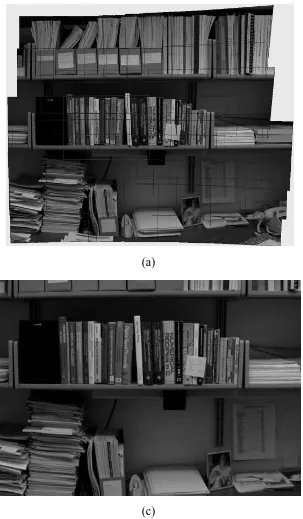
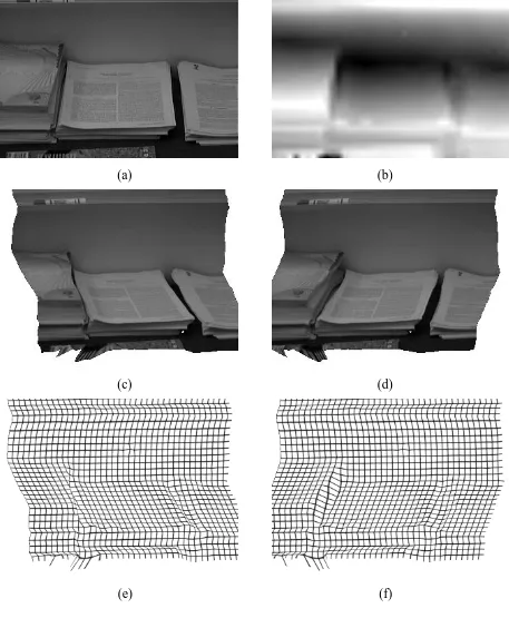
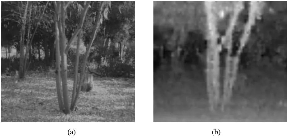
Figure 4 shows an example of using our projective depth recovery algorithm. The image sequence was taken by moving the camera up and over the scene of a table with stacks of papers (Figure 4a). The resulting depth-map is shown in Figure 4b as intensity-coded range values. Figures 4c–d show the original intensity image texture mapped onto the surface (an example of view extrapolation), and Figures 4c–d show a set of grid-lines overlayed on the recovered surface. The shape is recovered reasonably well in areas where there is sufficient texture (uniform intensity areas give no depth cues), and the extrapolated view looks reasonable. Figure 5a shows results from another sequence, this time from an outdoor scene of some trees. Again, the geometry of the scene is recovered reasonably well, as indicated in the depth map in Figure 5b.
7
Full 3-D model recovery
7 Full 3-D model recovery 15
(a) (b)
(c) (d)
[image:21.612.77.534.109.664.2](e) (f)
Figure 4: Depth recovery example: table with stacks of papers
16 7 Full 3-D model recovery
[image:22.612.73.542.89.313.2](a) (b)
Figure 5: Depth recovery example: outdoor scene with trees (a) input image, (b) intensity-coded depth map (dark is farther back).
side of an object, full 3-D models may be required. This is the most difficult image mosaicing problem, since not only do we have to recover depth, but we also have to merge (register and composite) multiple depth maps, and represent objects given no a priori knowledge about their rough shape or topology.
For simple topologies and shapes, deformable physically-based models can do a good job of recovering the unknown geometry [Terzopoulos et al., 1987; Pentland and Sclaroff, 1991]. For general topologies, the problem is more difficult. Since many current shape recovery techniques produce incomplete or sparse geometric descriptions, a general 3-D surface interpolation technique may be required to generate a smooth continuous surface [Hoppe et al., 1992; Szeliski and Tonnesen, 1992].
7 Full 3-D model recovery 17
(a) (b)
175
[image:23.612.68.565.146.645.2](c) (d)
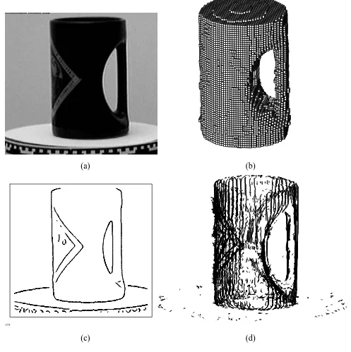
Figure 6: 3-D model recovery example
18 8 Applications
Our first technique converts each image into a binary silhouette by differencing the image with an empty background image. Each cube in the octree volumetric 3-D model is then projected (using the known camera position) into the silhouette, and cubes that fall outside the silhouette are culled. Cubes which fall partially into the silhouette are marked for later subdivision, and the process is repeated after each complete revolution at successively finer resolutions [Szeliski, 1993]. The resulting octree is shown in Figure 6b.
Our second technique extracts silhouette (extremal) edges from the image sequence, and uses a multi-frame stereo algorithm to reconstruct their 3-D position (internal albedo edges are also ex-tracted and reconstructed) [Szeliski and Weiss, 1993]. Figure 6c shows one of the edge images used by the algorithm, and Figure 6d shown the collection of 3-D curves estimated by the algorithm.
These examples demonstrate some of our algorithms for reconstructing an isolated object undergoing known motion. Similar techniques can be used to solve the more general 3-D scene recovery problem where the camera motion is unknown. Methods for determining the motion include the projective motion algorithm presented in the previous section, as well as techniques described in [Horn, 1986; Weng et al., 1993; Azarbayejani et al., 1993]. Compared to the 2-D and depth-map models developed in Sections 4–6, the recovery of 3-D models is more difficult and less robust, but holds the promise of more realistic and more general object and scene models.
8
Applications
Given automated techniques for building 2-D and 3-D scenes from video sequences, what can we do with these models? In this section, we describe a number of potential applications, including whiteboard and document scanning, 3-D model acquisition for inverse CAD, model acquisition for computer animation and special effects, supermarket shopping at home, interactive walkthroughs of historical buildings, and live tele-reality (telepresence) applications.
8.1
Planar mosaicing applications
8.2 3-D model building applications 19
1993] (see [Gold, 1993] for other examples of ubiquitous computing and augmented reality.) The techniques developed in this paper enable any video camera attached to a computer to be used. In specialized situations, e.g., in classrooms, a computer-controlled camera could be used to perform the scanning, removing the need for automatic registration of the images.
Another obvious application of this technology is for document scanning. Hand-held scanners currently perform this function quite well. However, since they are based on linear CCDs, they are subject to “skewing” problems in each strip of the scanned image which must be corrected manually. Using 2-D video images as input removes some of these problems. A final global skew may still be needed to make the document square, but this can be performed automatically by detecting document edges or internal horizontal and vertical edges (e.g., column borders).
8.2
3-D model building applications
The 3-D model building technology, while more difficult to automate reliably, has even greater potential. For example, we could construct a 3-D fax which would scan 3-D objects at one end using a video camera and either mechanical or user-controlled motion, and a 3-D graphics display at the other end [Carlbom et al., 1992]. This fax could be used to transmit 3-D models to a remote site for viewing and design revision, or to input rough CAD models for reverse engineering or clay mock-up applications. Of course, this technology could also be combined with stereolithography or numerically controlled milling to make this a true solid 3-D fax [Bresenham, 1993].
Rapid 3-D model building is also critical in the computer animation and special effects in-dustries. Currently, it can take days or weeks to build by hand each computer model used in a feature-length film. The ability to build such models rapidly from real objects or physical mock-ups would be of great utility, especially when freed from the range and resolution limitations of active rangefinding systems. The techniques we use for computing 3-D geometry could also be modified to automatically track the motions of objects or actors in a scene (this is called motion capture, and is currently done using specially placed markers.)
8.3
End-user applications
20 8 Applications
has the advantage of having a familiar look and organization, and enables the pre-planning of your next shopping trip. The images of the aisles (with their current contents) can be digitized by rolling a video camera through the store. More detailed geometric models of individual items can be acquired either by a 3-D model building process, or, in the future, directly from the manufacturer. The shopper can then stroll down the aisles, pick out individual items, and look at their ingredients and prices.
A similar scenario is possible with other buildings. Architectural walkthroughs have long been a part of computer graphics [Greenberg, 1974], but only for buildings currently under design. Walkthrough of existing building can have a number of applications. For example, interactive 3-D walkthroughs of your home, built by walking a video camera through the rooms and mosaicing the image sequences, could be used for selling your house (an extension of existing still-image based systems), or for re-modeling or renovating its design. Walkthroughs of historic building (e.g., palaces or museums) can be used for educational and entertainment purposes. A museum scenario might include the ability to look at individual 3-D objects such as sculptures, and to bring up related information in a hypertext system [Miller et al., 1991].
Walkthroughs (or fly-throughs) can also be done in general (e.g., outdoor) 3-D scenes. An early example of this was the Movie-Maps project [Lippman, 1980] which was based on videodisc tech-nology. Since this system was based on choosing from a number of pre-stored motion sequences, the range of possible viewpoints (and detail) was limited. The basic Movie-Maps idea can be extended by building true 3-D scenes from the input motion sequences. Such 3-D tele-reality models have the potential of being of extremely high complexity and will require solving problems in representation, partial 3-D models [Chen and Williams, 1993], and switching between different levels of resolution [Funkhouser and S´equin, 1993].
9 Discussion 21
(or special-purpose stereo hardware). In such applications, we need to use multiple cameras, since in moving scenes we cannot rely on the motion parallax from a single camera to give us reliable shape information.
9
Discussion
Image mosaicing provides a powerful new way of creating the detailed 3-D models and scenes needed for tele-reality applications. By registering multiple images together, we can create scenes of extremely high resolution and at the same time recover partial or full 3-D geometric information. While we use techniques from computer vision to perform the registration, our focus is different: traditional vision techniques are designed for inspection, recognition, and robot control, while our techniques are designed to produce realistic 3-D models for computer graphics and virtual reality applications.
The approach we use, namely direct minimization of intensity differences between warped images, has a number of advantages over more traditional vision techniques, which are based on tracking features from frame to frame [Tomasi and Kanade, 1992; Azarbayejani et al., 1993; Szeliski and Kang, 1994]. Our techniques produce dense estimates of shape, work in highly textured areas where features may not be reliably observed, and make statistically optimal use of all the information [Szeliski and Coughlan, 1994]. Our approach is similar to [Bergen et al., 1992], who also use intensity differences. However, we use full 2-D projective models of motion instead of instantaneous quadratic flow fields, and we also use a projective formulation of structure from motion, which eliminates the need for calibrated cameras. It is also very similar to [Mann, 1993], who also use planar projective motion estimates. Furthermore, [Mann and Picard, 1994] have also demonstrated superresolution results, i.e., the ability to obtain higher resolution images by simply jittering the camera rather than panning [Irani and Peleg, 1991].
22 10 Conclusions
accuracy (the results in this paper were obtained with uncalibrated cameras.)
The depth extraction techniques we use rely on the presence of texture in the image. In areas of sufficient texture, it is still possible for the registration/matching algorithm to compute an erroneous depth estimate (such gross errors are less common in active rangefinders.) Where texture is absent, interpolation must be used, and this can lead to erroneous (hallucinated) depth estimates. Other visual cues, such as occluding contours or shading [Horn, 1986], can be used to mitigate these problems in some cases, but a general-purpose reliable vision-based ranging system remains very much an open research problem.
The size and structure of the models produced for tele-reality applications have interesting implications for specialized graphics hardware and software interfaces. Current graphics hardware stores the intensity images (texture maps) separately from the geometry, which is stored as polygons usually spanning many pixels. A more appropriate architecture might be registered multi-resolution color images and depth maps. View interpolation, rather than 3-D rendering, could then be used to synthesize novel 3-D views [Chen and Williams, 1993]. These kinds of architectures and algorithms point towards a tighter coupling between computer graphics and image processing [Pickering, 1993].
10
Conclusions
10 Conclusions 23
Acknowledgements
Bob Thomas introduced me to the term tele-reality, which he used to describe the live concert telepresence scenario. James Coughlan developed the image registration code. David Tonnesen, Demetri Terzopoulos, Sing Bing Kang, and Richard Weiss were collaborators on some of the 3-D reconstruction algorithms described in this paper. William Hsu helped me produce the results in this paper. Ingrid Carlbom and Gudrun Klinker provided useful comments on the manuscript.
References
[Cyberware Laboratory Inc, 1990] Cyberware Laboratory Inc. 4020/RGB 3D Scanner with color
digitizer. Monterey, 1990.
[Adam, 1993] J. A. Adam. Virtual reality is for real. Spectrum, :22–29, October 1993.
[Azarbayejani et al., 1993] A. Azarbayejani, B. Horowitz, and A. Pentland. Recursive estimation of structure and motion using relative orientation constraints. In IEEE Computer Society
Conference on Computer Vision and Pattern Recognition (CVPR’93), pages 294–299, New
York, New York, June 1993.
[Ballard and Brown, 1982] D. H. Ballard and C. M. Brown. Computer Vision. Prentice-Hall, Englewood Cliffs, New Jersey, 1982.
[Barnard and Fischler, 1982] S. T. Barnard and M. A. Fischler. Computational stereo. Computing
Surveys, 14(4):553–572, December 1982.
[Beier and Neely, 1992] T. Beier and S. Neely. Feature-based image metamorphosis. Computer
Graphics (SIGGRAPH’92), 26(2):35–42, July 1992.
[Bergen et al., 1992] J. R. Bergen, P. Anandan, K. J. Hanna, and R. Hingorani. Hierarchical model-based motion estimation. In Second European Conference on Computer Vision (ECCV’92), pages 237–252, Springer-Verlag, Santa Margherita Liguere, Italy, May 1992.
[Beymer et al., 1993] D. Beymer, A. Shashua, and T. Poggio. Example Based Image Analysis and
Synthesis. A. I. Memo 1431, Massachusetts Institute of Technology, November 1993.
24 10 Conclusions
[Bresenham, 1993] J. Bresenham. Real virtuality: Stereolithography – rapid prototyping in 3-D.
Computer Graphics (SIGGRAPH’93), :377–378, August 1993.
[Brown, 1992] L. G. Brown. A survey of image registration techniques. Computing Surveys, 24(4):325–376, December 1992.
[Carlbom et al., 1992] I. Carlbom and others. Modeling and analysis of empirical data in collab-orative environments. Communications of the ACM, 35(6):74–84, April 1992.
[Carlbom et al., 1991] I. Carlbom, D. Terzopoulos, and K. M. Harris. Reconstructing and visual-izing models of neuronal dendrites. In N. M. Patrikalakis, editor, Scientific Visualization of
Physical Phenomena, pages 623–638, Springer-Verlag, New York, 1991.
[Chen and Williams, 1993] S. Chen and L. Williams. View interpolation for image synthesis.
Computer Graphics (SIGGRAPH’93), :279–288, August 1993.
[Dhond and Aggarwal, 1989] U. R. Dhond and J. K. Aggarwal. Structure from stereo—a re-view. IEEE Transactions on Systems, Man, and Cybernetics, 19(6):1489–1510, Novem-ber/December 1989.
[Earnshaw et al., 1993] R. A. Earnshaw, M. A. Gigante, and H. Jones, editors. Virtual Reality
Systems. Academic Press, London, 1993.
[Faugeras, 1992] O. D. Faugeras. What can be seen in three dimensions with an uncalibrated stereo rig? In Second European Conference on Computer Vision (ECCV’92), pages 563–578, Springer-Verlag, Santa Margherita Liguere, Italy, May 1992.
[Foley et al., 1990] J. D. Foley, A. van Dam, S. K. Feiner, and J. F. Hughes. Computer Graphics:
Principles and Practice. Addison-Wesley, Reading, MA, 2 edition, 1990.
[Funkhouser and S´equin, 1993] T. A. Funkhouser and C. H. S´equin. Adaptive display algorithm for interactive frame rates during visualization of complex virtual environments. Computer
Graphics (SIGGRAPH’93), :247–254, August 1993.
[Gleicher and Witkin, 1992] M. Gleicher and A. Witkin. Through-the-lens camera control.
Com-puter Graphics (SIGGRAPH’92), 26(2):331–340, July 1992.
[Gold, 1993] R. Gold. Ubiquitous computing and augmented reality. Computer Graphics
(SIG-GRAPH’93), :393–394, August 1993.
10 Conclusions 25
[Greene, 1986] N. Greene. Environment mapping and other applications of world projections.
IEEE Computer Graphics and Applications, 6(11):21–29, November 1986.
[Greene and Heckbert, 1986] N. Greene and P. Heckbert. Creating raster Omnimax images from multiple perspective views using the elliptical weighted average filter. IEEE Computer
Graph-ics and Applications, 6(6):21–27, June 1986.
[Hartley, 1994] R. I. Hartley. Euclidean reconstruction from uncalibrated views. In IEEE
Com-puter Society Conference on ComCom-puter Vision and Pattern Recognition (CVPR’94), Seattle,
Washington, June 1994.
[Hoppe et al., 1992] W. Hoppe and others. Surface reconstruction from unorganized points.
Com-puter Graphics (SIGGRAPH’92), 26(2):71–78, July 1992.
[Horn, 1986] B. K. P. Horn. Robot Vision. MIT Press, Cambridge, Massachusetts, 1986.
[Irani and Peleg, 1991] M. Irani and S. Peleg. Improving resolution by image registration.
Graph-ical Models and Image Processing, (3), May 1991.
[Jepson and Black, 1993] A. Jepson and M. J. Black. Mixture models for optical flow computa-tion. In IEEE Computer Society Conference on Computer Vision and Pattern Recognition
(CVPR’93), pages 760–761, New York, New York, June 1993.
[Kuglin and Hines, 1975] C. D. Kuglin and D. C. Hines. The phase correlation image alignment method. In IEEE 1975 Conference on Cybernetics and Society, pages 163–165, New York, September 1975.
[Lippman, 1980] A. Lippman. Movie maps: An application of the optical videodisc to computer graphics. Computer Graphics (SIGGRAPH’80), 14(3):32–43, July 1980.
[Mann, 1993] S. Mann. Compositing multiple pictures of the same scene: Generalized large-displacement 8-parameter motion. In Proceedings of the 46th Annual IS&T Conference, The Society of Imaging Science and Technology, Cambridge, Massachusetts, May 1993.
[Mann and Picard, 1994] S. Mann and R. W. Picard. The projective group model for multi-frame resolution enhancement. In First IEEE International Conference on Image Processing
(ICIP’94), (submitted) 1994.
[Matthies et al., 1989] L. H. Matthies, R. Szeliski, and T. Kanade. Kalman filter-based algorithms for estimating depth from image sequences. International Journal of Computer Vision,
26 10 Conclusions
[Miller et al., 1991] G. Miller and others. The virtual museum: Interactive 3D navigation of a multimedia database. Journal of Visualization and Computer Animation, 3(3):183–198, 1991.
[Moffitt and Mikhail, 1980] F. H. Moffitt and E. M. Mikhail. Photogrammetry. Harper & Row, New York, 3 edition, 1980.
[Okutomi and Kanade, 1993] M. Okutomi and T. Kanade. A multiple baseline stereo. IEEE
Transactions on Pattern Analysis and Machine Intelligence, 15(4):353–363, April 1993.
[Pentland and Sclaroff, 1991] A. Pentland and S. Sclaroff. Closed-form solutions for physically-based shape modeling and recognition. IEEE Transactions on Pattern Analysis and Machine
Intelligence, 13(7):715–729, July 1991.
[Pickering, 1993] W. R. Pickering. Merging 3-D graphics and imaging – applications and issues.
Computer Graphics (SIGGRAPH’93), :395–396, August 1993.
[Porter and Duff, 1984] T. Porter and T. Duff. Compositing digital images. Computer Graphics
(SIGGRAPH’84), 18(3):253–259, July 1984.
[Press et al., 1992] W. H. Press, B. P. Flannery, S. A. Teukolsky, and W. T. Vetterling. Numerical
Recipes in C: The Art of Scientific Computing. Cambridge University Press, Cambridge,
England, second edition, 1992.
[Quam, 1984] L. H. Quam. Hierarchical warp stereo. In Image Understanding Workshop, pages 149–155, Science Applications International Corporation, New Orleans, Louisiana, December 1984.
[Rehg and Kanade, 1994] J. Rehg and T. Kanade. Visual tracking of high dof articulated structures: an application to human hand tracking. In Third European Conference on Computer Vision
(ECCV’94), pages 35–46, Springer-Verlag, Stockholm, Sweden, May 1994.
[Rioux and Bird, 1993] M. Rioux and T. Bird. White laser, synced scan. IEEE Computer Graphics
and Applications, 13(3):15–17, May 1993.
[Semple and Kneebone, 1952] J. G. Semple and G. T. Kneebone. Algebraic Projective Geometry. Clarendon Press, Oxford, England, 1952.
[Szeliski, 1991] R. Szeliski. Shape from rotation. In IEEE Computer Society Conference on
Com-puter Vision and Pattern Recognition (CVPR’91), pages 625–630, IEEE ComCom-puter Society
10 Conclusions 27
[Szeliski, 1993] R. Szeliski. Rapid octree construction from image sequences. CVGIP: Image
Understanding, 58(1):23–32, July 1993.
[Szeliski, 1994] R. Szeliski. A least squares approach to affine and projective structure and motion recovery. 1994. In preparation.
[Szeliski and Coughlan, 1994] R. Szeliski and J. Coughlan. Hierarchical spline-based image reg-istration. In IEEE Computer Society Conference on Computer Vision and Pattern Recognition
(CVPR’94), Seattle, Washington, June 1994.
[Szeliski and Kang, 1994] R. Szeliski and S. B. Kang. Recovering 3D shape and motion from image streams using nonlinear least squares. Journal of Visual Communication and Image
Representation, 5(1):10–28, March 1994.
[Szeliski and Tonnesen, 1992] R. Szeliski and D. Tonnesen. Surface modeling with oriented par-ticle systems. Computer Graphics (SIGGRAPH’92), 26(2):185–194, July 1992.
[Szeliski and Weiss, 1993] R. Szeliski and R. Weiss. Robust shape recovery from occluding con-tours using a linear smoother. In Image Understanding Workshop, pages 939–948, Morgan Kaufmann Publishers, Washington, D. C., April 1993. A longer version is available as CRL TR 93/7.
[Terzopoulos and Witkin, 1988] D. Terzopoulos and A. Witkin. Physically-based models with rigid and deformable components. IEEE Computer Graphics and Applications, 8(6):41–51, 1988.
[Terzopoulos et al., 1987] D. Terzopoulos, A. Witkin, and M. Kass. Symmetry-seeking models and 3D object reconstruction. International Journal of Computer Vision, 1(3):211–221, October 1987.
[Tomasi and Kanade, 1992] C. Tomasi and T. Kanade. Shape and motion from image streams under orthography: A factorization method. International Journal of Computer Vision, 9(2):137–154, November 1992.
[Wang and Adelson, 1993] J. Y. A. Wang and E. H. Adelson. Layered representation for motion analysis. In IEEE Computer Society Conference on Computer Vision and Pattern Recognition
(CVPR’93), pages 361–366, New York, New York, June 1993.
[Wellner, 1993] P. Wellner. Interacting with paper on the DigitalDesk. Communications of the
28 A 2-D projective transformations
[Weng et al., 1993] J. Weng, T. S. Huang, and N. Ahuja. Motion and Structure from Image
Sequences. Springer-Verlag, Berlin, 1993.
[Witkin et al., 1987] A. Witkin, D. Terzopoulos, and M. Kass. Signal matching through scale space. International Journal of Computer Vision, 1:133–144, 1987.
[Wolberg, 1990] G. Wolberg. Digital Image Warping. IEEE Computer Society Press, Los Alami-tos, California, 1990.
A
2-D projective transformations
Planar scene views are related by projective transformations. This is true in the most general case, i.e., for any 3-D to 2-D mapping,
u
=M
camp
(14)where
p
is a 3-D world coordinate,u
is the 2-D screen location, andM
camis a 34 camera matrixdefined in (4). Since
M
camis of rank 3, we havep
=M
u
+
s
m
(15)where
M
is a left inverse of
M
cam andm
is in the null space ofM
cam, i.e.,M
camm
= 0. Theequation of a plane in world coordinates can be written as
ax
+by
+cz
=d
orn
p
=0 (16)from which we can conclude that
n
TM
u
+
s
n
m
=0 ors
=;(n
TM
u
)
=
(n
m
) (17)and hence
p
=(I
;(n
m
);1
mn
T )M
u
=
Mu
˜:
(18)From any other viewpoint, we have
u
0 =M
0
cam
Mu
˜ =M
2Du
(19)A 2-D projective transformations 29
For the remainder of this appendix, it is convenient to assume that the world coordinate system coincides with the first camera position, i.e.,
E
=I
andM
cam =V
=h
ˆ
V 0
i, and therefore
M
=ˆ
V
;1and
m
= (0001) Tin (15–18). An image point
u
then corresponds to a world coordinatep
,p
= 24
ˆ
V
;1u
w
3
5
(20)where
w
is the unknown fourth coordinate ofp
(called projective depth) which controls how far the point is from the origin.For panoramic image mosaicing, we rotate the point
p
around the camera optical center to obtainp
0 =2
4
R 0
0
T 1 3 5p
= 2 4R
ˆV
;1u
w
3
5
(21)with a corresponding screen coordinate
u
0 =ˆ
V
0R
V
ˆ;1u
=
M
2Du
:
(22)Thus, the mapping between the two screen coordinate systems can be described by a 2-D projective transformation.
For piecewise-planar scenes, the point
p
will lie on some planek
whose equation we can write asn
kp
=(n
ˆ k;1)
p
=0.6 Then, (18) reduces to
p
k = 2 4I
n
T k 35
V
ˆ ;1u
(23)
as the 3-D position on plane
k
corresponding to the screen positionu
. In a second camera position, the world coordinates have undergone a Euclidean transformationp
0k =
Ep
k with rotation
R
andtranslation
t
. The new screen coordinates are thereforeu
0 k =V
0Ep
k = ˆV
0(
R
+tn
T k )ˆ
V
;1u
=M
k
u
(24)Thus, we see that 2-D projective motion matrices for the various planar pieces are interrelated, and are in fact determined by the plane equations (
n
k), the rigid motion (R
andt
), and the viewingmatrices ( ˆ
V
and ˆV
0). For methods for recovering these unknown parameters from the
M
k, see[Faugeras, 1992; Hartley, 1994].
30 A 2-D projective transformations
For general depth recovery, each image point
u
corresponds to a 3-D pointp
with an unknown projective depthw
as given in (20). In some other frame, whose relative orientation to the first frame is denoted byE
, we haveu
0 =V
0
Ep
=ˆ
V
0R
V
ˆ;1u
+w
ˆ
V
0t
=
M
2Du
+w
t
ˆ:
(25)Thus, the motion between the two frames can be described by our familiar 2-D planar projective motion, plus an amount of motion proportional to the projective depth along the direction ˆ
t
(which is called the epipole) [Faugeras, 1992]. Note that the values ofM
2D, ˆt
, andw
are notunique: there is a scale ambiguity between
w
and ˆt
, and multiples of ˆt
can be added toM
2Dwith the appropriate adjustments to
w
. To remove these ambiguities, we must enforce the rigidity constraintsM
2D =V
ˆ0