6
I
January 2018
Fuzzy Methods for Soft Hidden Markov Modelling
J. Rama1, S. Rajakumari2, K.Visalakshi3, S.Ananthi4 1
Department of Network Systems and Information Technology, University of Madras, India, 2,3Dr.Dharmambal Polytechnic College for Women, Taramani, India,
4
Department of Network Systems and Information Technology, University of Madras, India,
Abstract: The use of fuzzy logic has no limits in for its power to solve real life problems either for control or for information. In the realm of information transfer through coding schemes, there are certain probabilistic algorithms currently in use very much for digital communications. To examine the feasibility of rethinking one of these problems based on the fuzzy logic principle has been considered. For this purpose, the principles relating to the basic hidden Markov Model has been discussed. The model is explained with an example in a lucid manner and the three problems associated with the solution of such models is brought out, with an example on speech recognition as well, given in the appendix, as drawn from current recent literature. Speech recognition in a computer system domain may be defined as the ability of computer systems to accept spoken words in an audio
format - such as wav or raw and then generate its content in text format. Speech recognition in a computer domain involves various steps with issues attached with them. In this paper, we focus on tackling these various issues while implementing a speaker-independent.
Keywords: Hidden Markov Model, Viterbi algorithm, GSM, Fuzzy Logic, Baum-Welch algorithm.
I. INTRODUCTION
A discrete time discrete space dynamical system governed by a Markov chain emits a sequence of observable outputs, one output for each state in a sequence (time) of such states. From the observed outputs, to infer the most likely dynamical system is a motivation for many physical signals. This results in a model for the underlying process alternatively, given a sequence of outputs; infer the most likely sequence of inputs or states. The model can also be used to foretell the next observation or more generally a sequence of them. The contents of this chapter are meant to illustrate how fuzzy logic is simpler to understand than the usually dealt with technique of Viterbi decoding. In essence, both do the same function and perhaps, the inner aspects of the algorithm are covered by the simpler exposition of a fuzzy logic based method. Convolutional code is generated by combining the outputs of a K-stage shift register by using a number of exclusive OR summers. The method is very much in use in GSM communication of speech and data. Optimal encoding schemes have been worked out, giving the number K of shifts and the number v of adders and the manner of connections to the adders from the shift registers. Since for every bit, additional v bits are transmitted, there is good scope for error detection and correction. This paper is organized as follows. Section 2 comprises the implementation details for the system. The various algorithms and techniques used and the modifications suggested are discussed in this section. Section 3 describes the database development and the recognition procedure used. A discussion of the results obtained with testing the system with the above-mentioned database is presented in Section 4. Section 5 outlines the conclusions. Suggestions for improvement in the recognition accuracy of this experimental system are also presented in this section.
A. Hidden Markov Model (HMM)
State is a condition presently in. Input is a variable from time to time. A new input moves the current state to a different state. Every state transition has a probability. For example, from state 1 to state 2, it can be 100% probable. Then, any new input will only move state 1 to state 2. In some cases, from state 1, it can have 50% probability to reach state 1 or state 2, either being plausible. Then, it might move to state 1 or to state 2.
The output (observation) is dependent on present input and present state. Each such state can emit one or other data for observation. Suppose there could be four such data (observed outputs) possible; then one or two of these will have equal probability. The rest can have only zero probability.
Consider the rain-sun analog. Input today can be sun or rain. The state can have four values: sun-sun; rain-sun; rain-rain; sun-rain. That means, two days information makes a ‘state’. (This is a HMM of order 1).
Let it be rain the next day. Then, state 1 changes to (rain-sun) or state 2. So, state 1can only change to state 1 or state 2, for any input. Thus there is 50% fuzziness for transition from state1 to state 2, as also from state 1 to state 1 itself. However, for state 1 to 3 and 1 to 4 , there is no probability.
Next, consider the ‘Emission probabilities’ for observed results. We observe that if it changes from sun to sun, a person goes out of his house (sports, shopping, or whatever).If it changes from sun to rain, he remains inside. One can be doing some cleaning or gardening work also.
Table1
Present state State type Input type Observation
State 1 sun-sun sun/rain Outing/cleaning
State 2 rain-sun sun/rain gardening/cleaning
State 3 rain-rain sun/rain cleaning/gardening
State 4 sun-rain sun/rain outing/gardening
If one knows the sequence of observations of what happens (or one does) on every day, the sequence of input (the weather sun-rain-rain pattern) can be determined. This is the well known Alice and Bob conversation, who live in different regions of America, talking over a telephone line as to, what he did that day to Alice’. For each state, there is one observed fact, of which there are four. Suppose we know at start it has been sun for two days. So, starting state is 1. Then, the observation on subsequent day was gardening. Is it possible? No, because, at state 1, either an input of sun or rain, cannot have ‘gardening’ as an event. (It could be ‘outing’ or ‘cleaning’ only). We can designate these observed data as d1, d2,d3, d4. This is an error in observation perhaps. Even if there is an observed error, it shows up clearly. Figure.1 Shows the State transition probabilities at State no.1.
Fig. 1 State transition probabilities at State no.1.
At any day, the state is fixed, based on previous weather. (State 1 means sunny-sunny). There are two probabilities involved. One is the state to state change probability. From State 1 to state 1 or state 2 is fully probable. But not to states 3 and 4. Given day1 state as 1, state transition probabilities are 50,50,0,0.
Then there is another probability namely the emission probability of observations (outputs).
At state 1, their emission probabilities for the possible data are again dependent . If the four data are d1, d2, d3 ,d4, then from state 1, d1 ,d2 are fully (equally) probable, but d3,d4 have only a zero probability. Fig 2. Shows the Emission probability values for four data output from state 1.
Consider a set of such input data and the resulting observations as:
i1, i2,….. d1, d2,…….Given d1,d2…, finding i1,i2… is one form of the HMM problem. Here the model must be known to the observer. By this it is meant that the relations of state to state transition probabilities, and the state emission probabilities for all the inputs are known to the observer. This is also called a decoding problem.
In another HMM problem, the information of input i’s and observed d’s are both known. Also, the order of the HMM and the
ranges of i's and d’s are known. (By order we mean how many sequential values determine a state). (By range, we mean how many
possible inputs and outputs are likely; in the weather case, the i range is 2 (Rain and Sun) and the d range was 4. For a set n of data, the system is fully determined just by knowing the states. The group of states is shown on a diagram called the “Trellis”, much like a garden trellis.
Fig.3 shows the trellis diagram
By knowing the true state values at every point in the sequence the data input stream is found.
There is a proposition called “Dynamic programming”(Bellman .R,2003) . If we knew the correct state at any day (or time slot), any further state is determinable only by the input data. The states previous to this need not be known. A Markov process also means the same.
Therefore, knowing the correct occupied state numbers on every time slot determines the entire data. But if there is ambiguity in knowing the state (at anyone or more timeslots), then, the problem is to fix the better of the states among the group.
If there are two possible states at t=t1, then further on, at t+1, t+2 etc., there will be further ambiguities in determining the exact
states. Since one state leads to one or more possible states, the ambiguous state will lead to two ambiguous states in the next. After t+2, t+3 … there it is likely all (four in this case) states can be having values of truth different among them. So, this is thought of as a fuzzy logic problem. In fuzzy logic theory alone there is scope for admitting all possibilities as being admissible, each with its own degree of membership.
If we use the data stream to determine the fuzzy member values for each state from time to time, we will get a trellis of states, showing these values somewhat as in fig.4.
Fig.4. Showing memberships for all states for all time slots.
The figure 4 indicates the memberships for all states, starting from fully true state 1.
A defuzzification by the (max) principle will produce a diagram that fixes the (best) actual states. Thus, we summarise the above discussions in a mathematical formulation.
B. Three Basic Problems of HMM
C. The Evaluation Problem
Given an HMM and a sequence of observations
O = o1 , o2 , …,oT, ..(1)
what is the probability that the observations are generated by the model, P{O|}?
D. The Decoding Problem
Given a model and a sequence of observations
O = o1 , o2 , …,oT, …(2)
what is the most likely state sequence in the model that produced the observations?
E. The Learning Problem
Given a model and a sequence of observations
O = o1 , o2 , …,oT , how should we adjust the model parameters { , B, } in order to maximize P{O|}?
Evaluation problem can be used for isolated (word) recognition. Decoding problem is related to the continuous recognition as well as to the segmentation. Learning problem must be solved, if we want to train an HMM for the subsequent use of recognition tasks.
F. The Decoding Problem and the Viterbi Algorithm
In this case we want to find the most likely state sequence for a given sequence of observations, O = o1 , o2 , …,oT and a model,
= { , B, } . …(3) The solution to this problem depends upon the way “most likely state sequence'' is defined. One approach is to find the most likely state yt at t=t and to concatenate all such yt’ 's. But some times this method does not give a physically meaningful state sequence.
Therefore we would go for another method which has no such problems.
For decoding a HMM model, Viterbi algorithm is the standard prescribed method. This did not take any fuzzy logic technique into
consideration, perhaps because Viterbi’s original work was much earlier than when Fuzzy logic was proposed by Zadeh. Even till today, the principle by which F.L. can be exploited for our problem has not been considered either adjunct or separately to this famous algorithm. Since the Viterbi algorithm evolved around digital communication scheme using a technique called “convolutional coding”, for error free data reception, let us likewise consider the principle fo applying F.L. to this very same problem.
So, in the rest of this chapter, a review is presented for convolutional decoding and the Viterbi’s method also in a short form, as reported by vendor manuals offering this for Communication hardware products.
In this Viterbi algorithm, the whole state sequence with the maximum likelihood is found. In order to facilitate the computation we
define an auxiliary variable,
...(4) which gives the highest probability that partial observation sequence and state sequence up to t=t can have, when the current state is i.
It is easy to observe that the following recursive relationship holds.
( a & b being the two probabilities defined earlier) …(5)
where,
1(j) = j bj(o1) , 1 j N
So the procedure to find the most likely state sequence starts from calculation of T ( j ), , 1 j N using recursion in the above
equation,, while always keeping a pointer to the ``winning state'' in the maximum finding operation. Finally the state j*, is found
where
and starting from this state, the sequence of states is back-tracked as the pointer in each state indicates. This gives the required set of states.
This whole algorithm can be interpreted as a search in a graph whose nodes are formed by the states of the HMM in each of the time instant t, 1 t T.
Subsequent to this, let us consider the technique for applying F.L. principles to decode the transmitted data. A comparison of the techniques will enlighten one on the simplicity of the FL, a powerful technique that it is.
II. THE HMM RECOGNITION PROBLEM – SPEECH RECOGNITION
For this, let us see how the HMM is found to be of use. Each spoken word consists of sounds of literals, phonemes and soft white noise. The model here is one for each word. A word say “Thanks” will have a sequence of outputs which are one or more of these components. What comes as a sound is the observed output of the model. What is input is the word itself, which is a spoken signal. What the model has in it is the sound bits that it receives.
Here the problem is a learning problem first. They would submit a series of such “Thanks” to the model to identify its inner states, their number and the probabilities of state transitions and those of the emission of sound. The model is totally hidden, but it can be found by repeated observations of the same sound.
Usually, the observed data is not just the sound; it cannot be used for analyzing the model and estimating it. They use some other transform based information based on the sound, such as a logarithmic frequency domain plot. Since a frequency domain plot will not differentiate small changes on starting time and ending time of the spoken word, there will be the same spectral information that will result for almost all the time “Thanks” is spoken. That means, the observed data is almost the same for each utterance. In this manner, for a list of words, if the models are determined, then, when any one word is spoken, it can be analysed to find to which of these models that spoken word will fit best.
Fig.5. Shows the representation of the spoken word with respect to the Model.
This can be solved by the EM algorithm. The same is also possible by fuzzy logic techniques, but in our work, only the decoding problem is concentrated upon. The details of the method are given below in detail. Speech recognition in a computer system
domain may be defined as the ability of computer systems to accept spoken words in an audio format - such as wav or raw and then
generate its content in text format. Speech recognition in a computer domain involves various steps with issues attached with them. In this paper, we focus on tackling these various issues while implementing a speaker-independent, isolated Hindi word recognizer. A mention about the reason for choosing Hindi language is required here. Firstly, it is a language of local relevance. Hindi is the national language of India and is widely spoken in various parts of the country. The alphabets of the Hindi language themselves form the phoneme-set i.e., there is no separate phoneme-set unlike the English language. Besides, the Hindi alphabet is very well categorized on the basis of similarities in articulation methods of its letters. This property of Hindi makes it free of homonyms thus reducing the complexity of handling them in design of speech recognition systems. These advantages are more prominent in the case of phoneme-based recognizers, where a phonetic dictionary is not required for speech to text conversion.
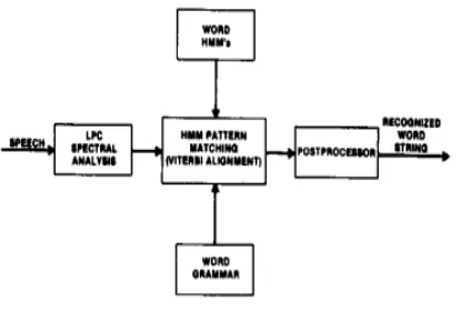
A. Design and Implementation
Figure 6 describes the structure of the word recognizer. The system can be run in two modes - training mode and testing mode. The system initially runs in the training mode for training the HMM for each word. Word recognition is performed in the testing mode. Each mode consists of the following three modules: (1) pre-processing of audio input and feature extraction using LPC and MFCC , (2) conversion of feature vectors into codebook indices using VQ and (3) recognition using HMM.
Fig. 6. describes the structure of the word recognizer
B. Pre-processing and Feature Extraction
Read wav fileThe speech signal is stored in the form of wave files and is read. The speech samples thus obtained are stored for further computations. The digitized (sampled) speech signal s(n) is put through a low-order digital system to spectrally flatten the signal. The first-order filter used had the transfer function H(z) = 1 - az-1 where a = 0.9375.
In Frame Blocking step, the pre-emphasized speech signal is blocked into frames of N samples, with adjacent frames being separated by M samples. Frame blocking is carried out to reduce the mean squared prediction error over a short segment of the speech wave form. In our case, N = 256 and M = 128. Features get periodically extracted. The time for which the signal is considered for processing is called a window and the data acquired in a window is called a frame. The window duration is 16ms. Thus, two consecutive frames have overlapping areas. We use a Hamming window for this purpose.
W(n) = 0.54 - 0.46cos(2 *pi*n/N -1) …(7)
0 (symbol of less than or equal to) n (symbol of less than or equal to) N-1
C. Noise and Silence Detection
Noise detection is performed using the energy threshold value and silence detection is performed using the zero crossing rate. The energy level of the signal is calculated using auto-correlation analysis of each frame. The average energy level and zero crossing rate of these frames are calculated and assigned as minimum threshold level and maximum zero crossing level. Only those frames which have an energy greater than the minimum threshold and a zero crossing rate less than the maximum set level are considered for further processing.
D. LPCC and MFCC Extraction
The next processing step is the LPC analysis, which converts each frame of p +1 autocorrelations (found from autocorrelation analysis in the previous step into an LPC parameter set by using DURBIN's method. Cepstral coefficients are the coefficients of the Fourier transform representation of the log magnitude spectrum. In our case, each frame is represented by 12 Cepstral and 12 delta-cepstral values. MFCC is considered to be the best available approximation of the human ear. It is known that the human ear is more sensitive to a higher frequency. The spectral information can be converted to MFCC by passing the signals through band pass
filters, where higher frequencies are artificially boosted, and then doing an inverse Digital Fourier Transform on it. This results in higher frequencies being more prominent. We obtained 20 MFCC coefficients for each frame of speech signal.
E. Vector Quantization
quantizing them. VQ is potentially an extremely efficient representation of spectral information in the speech signal. Assume that we have a set of L training vectors and we need a codebook of size M , we have used the K -means clustering algorithm, which can be summarized as Initialization: arbitrarily choose M vectors (we can choose these from the training set) as the initial set of code words in the codebook. Nearest-neighbor search: for each training vector, a codeword is found in the current codebook that is closest in terms of spectral distance, and assigns that vector to the corresponding cell.
Centroid update: update the codeword in each cell using the centroid of the training vector assigned to the cell. The distance measure used is the Euclidian Distance, whose minimum value is used to update the centroid. c (k) is the current centroid of the kth cluster and v ( k ) is a vector in the cluster. The result of the clustering is a codebook of size 128 (optimum size obtained from comparative testing). This is a universal codebook created by concatenating all feature vectors obtained from every utterance present in the database and clustering them. The codebook indices are used to obtain the observation symbols to be used in training and testing the HMM.
F. Recognition Using HMM
The HMM is a doubly stochastic process in which there is an unobservable Markov chain, each state of which is associated with a probabilistic function characterized by a probability distribution or a density function. The Markov chain is defined by a state transition matrix, while the probabilistic function, designated as the observation probabilities or densities, may be a non-parametric or non-parametric representation . In isolated word recognition using the Markovian modeling, there are two phases: the training phase and the recognition phase. In the training phase, a training set of observations are used to derive a set of reference models. In the recognition phase, the probability of generating the test observation is computed for each reference model. The test utterance is classified as the word whose model gives the highest score.
The model is characterized by the following elements, the number of states in a model. In speech recognition context, there are two methods to estimate the value of N..
States which represent a phonetic entity (phonemes, phones, syllables).
States which represent temporal frames. M, the number of observation symbols per state. It is the discrete alphabet size.
A = { a ij}, is the state transition probability matrix and a ij represents the probability of making a transition to state j, given that the model is in state i.
B ={ b i ( k )}, is the model output symbol probability matrix, where b i ( k ) represents the probability of outputting the symbol k , given that the model is in the state i .
∏= {πi} is the initial state probability vector. In the speech recognition context, we assume that the system always begins in the state 1.
With an appropriate value of N,M,A,B, ∏, the HMM can be used to generate the observation sequence O=O 1 O 2...OT . These
sequences are used as both a generator of observations and as a model for how a given observation sequence was generated by an appropriate HMM. Optimal state sequence to produce given observations, O={o1,…,ok} and given model. The solution to this problem in reference to word recognition is done using the Viterbi search. Determine the optimum model, given a training set of
observations O, find λ, such that P(O/λ) is maximal. This is done to re-estimate the parameters of each HMM. For a particular word, 35 utterances of the word are used to re-estimate the parameters using the Baum-Welch algorithm.
G. Database Development and Recognition
Data set used for experiments
Number of speakers - 35 (20 M + 15 F) Language used - Standard Hindi
Average duration of training and testing utterance - 500-800 msec. Audio recording - S/N >40 db
Sampling and quantization - 16.025 kHz, 16 bits; Recognition stage can be formulated in the following way: The utterance of an unknown word is analyzed and we obtain an observation sequence of acoustic vectors.
Each vector of the sequence is transformed into a symbol, which is the index in the codebook corresponding to the prototype that matches the best initial vector. Finally, the sequence of vectors is replaced by a symbolic chain. For the observation sequence of
III. THE DATA DECODING PROBLEM IN DIGITAL COMMUNICATION
The use of some form of error correcting code is common in digital communications that we handle in every day life. Among these, the GSM and many other schemes employ the so called convolutional coding [9], [10], [11]. This code is a redundant code, because for sending n data, the method will use 2 n data or more. The use of redundancy enables errors to be fixed.
For the purpose of generating the redundant code from the actual digital data, the same uses a Markov model, with a delay chain. The data symbols are kept stored for 2 or 3 time units, using delay lines or memory. Then, the output data (the observe data or the actually transmitted data) is made up of a combination of the memory symbols, as per any logical equation. Such a logical equation could be, say, just adding two past data symbols to the current input to yield one observed bit value. For every bit of input, there will be two or three or more bits output, depending upon the redundancy employed. Usually, as in GSM communication, every bit is transformed to two bits. These two bits are obtained by a certain logical combination of the input bit and some of the past bits, kept stored in memory or delay lines (fig.6).
Fig.6 shows the logical combination for the given nput data
Here, the model is predetermined. That is, the coding scheme defines the model. For GSM, there is a model; for another, a different model and so on.
Since the model is known in this case, the data is unknown, while the observed bits are the transmitted information. The method of finding the original data is called “decoding the data received”. This problem is of great importance in today’s communication requirements.
Andrew Viterbi was the originator of the algorithm that goes by his name and that is what is employed in the digital communication codecs today. This whole algorithm can be interpreted as a search in a graph whose nodes are formed by the states of the HMM in each of the time instant.
IV. CONCLUSION
The use of the Hidden Markav Model (HMM) for recognition and decoding applications with the elements of fuzzy logic combined is usual decoding algorithms described in this paper. This technique helps in a soft method of usage of the said model for any applications including digital communication.
REFERENCES
[1]. Asghar.Taheri ,”Fuzzy Hidden Markov Models for Speech Recognition on based FEM Algorithm”, Proceedings Of World Academy Of Science, Engineering And Technology Volume 4 February 2005.ISSN 1307-688
[2]. Babuška, R. (1998), Fuzzy Modeling and Identication Toolbox For Use with Matlab, User's Guide, Control Engineering Laboratory, Delft University of Technology, The Netherlands.
[3]. Bansal P, Dev A, Jain SB., “Optimum HMM combined with vector quantization for hindi speech word recognition”,IETE J Res, 54:239-43, 2008. [4]. Bellman .R, “Dynamic Programming”, Dover Publications Inc, UK, 2003
[5]. Asghar.Taheri ,”Fuzzy Hidden Markov Models for Speech Recognition on based FEM Algorithm”,Proceedings Of World Academy Of Science, Ngineering And Technology Volume 4 February 2005.ISSN 1307-688
[6]. Babuška, R. (1998), Fuzzy Modeling and Identification Toolbox For Use with Matlab, User's Guide, Control Engineering Laboratory, Delft University of Technology, The Netherlands.
[7]. Bansal P, Dev A, Jain SB., “Optimum HMM combined with vector quantization for hindi speech word recognition”,IETE J Res, 54:239-43, 2008. [8]. Bellman .R, “Dynamic Programming”, Dover Publications Inc, UK, 2003
[9]. Rabiner.L.R & Juang .B.H, Fundamentals of speech recognition, Prentice Hall of India, Prentice Hall (Signal Processing Series), 1993.
[10]. Bahi. H. & Sellami M, Combination of vector quantization and hidden Markov models for Arabic speech recognition, Proceedings ACS/IEEE International conference on computer systems and applications, Beirut, Lebanon, pp. 96-100, June 2001.
[12]. http://www.ece.ucsb.edu/Faculty/Rabiner/ece259/Reprints
[13]. Shannon & Paliwal, B.J. Shannon & K.K. Paliwal, MFCC Computation from Magnitude Spectrum of higher lag autocorrelation coefficients for robust speech recognition, Proceedings of ICSLP (2004), pp. 129-132.
[14]. Chulhee Lee, Donghoon Hyun, Euisun Choi, Jinwook Go & Chungyoung Lee, 'Optimizing feature extraction for speech recognition', IEEE Transactions on Speech and audio processing , Vol. 11, No.1, January 2003.
[15]. Poonam Bansal, Amita Dev & Shail Bala Jain, 'Enhanced feature vector set for VQ recogniser in isolated word recognition', Proceedings of Intenational conference on Information Research & Applications , iTech 2007,Verna, Bulgaria, pp. 390-395, June 2007.
[16]. Rabiner.R, Levinson.S.E, & Sondhi M.M,, 'On the application of Vector Quantization and Hidden Markov Models to speaker independent, isolated word recognition', The Bell System TechnicalJournal , Vol. 62, No. 4, April 1983.