Master's Theses (2009 -) Dissertations, Theses, and Professional Projects
Applying Bayesian Forecasting to Predict New
Customers' Heating Oil Demand
Tsuginosuke Sakauchi
Marquette University
Recommended Citation
Sakauchi, Tsuginosuke, "Applying Bayesian Forecasting to Predict New Customers' Heating Oil Demand" (2011).Master's Theses (2009 -).Paper 108.
by
Tsuginosuke Sakauchi, B.S.
A Thesis Submitted to the Faculty of the Graduate School, Marquette University, in Partial Fulfillment of the Requirements for
the Degree of Master of Science
Milwaukee, Wisconsin August 2011
HEATING OIL DEMAND
Tsuginosuke Sakauchi, B.S. Marquette University, 2011
This thesis presents a new forecasting technique that estimates energy
demand by applying a Bayesian approach to forecasting. We introduce our Bayesian Heating Oil Forecaster (BHOF), which forecasts daily heating oil demand for
individual customers who are enrolled in an automatic delivery service provided by a heating oil sales and distribution company. The existing forecasting method is based on linear regression, and its performance diminishes for new customers who lack historical delivery data. Bayesian methods, on the other hand, respond effectively in the start-up situation where no prior data history is available.
Our Bayesian Heating Oil Forecaster uses forecasters’ past performances for existing customers to adjust the current forecast for target customers. We adapted a Bayesian approach to forecasting combined with domain knowledge and original ideas to develop our Bayesian Heating Oil Forecaster, which forecasts demand for target customers without relying on their historical deliveries.
Performance evaluation demonstrates that our Bayesian Heating Oil
Forecaster shows increased performance over the existing forecasting method when the two techniques are combined. We used Root Mean Squared Error (RMSE) and Mean Absolute Percent Error (MAPE) to compare the performance of the two algorithms. Compared to the existing forecasting method alone, our Simple Average model, which combines the forecasts from the existing forecasting method and our Bayesian Heating Oil Forecaster, recorded an overall improvement of 2.4% in RMSE, 5.0% in MAPE Actual, and 2.8% in MAPE Capacity for company A and 0.3%, 7.1%, and 2.8% for company B.
ACKNOWLEDGMENTS
Tsuginosuke Sakauchi, B.S.
The completion of this thesis would have been impossible without the extensive encouragement and guidance I received from my mentors, colleagues, and my family. I would like to specifically express my sincere gratitude to Dr. Brown and Dr. Corliss. Dr. Brown offered profound technical insights from the energy forecasting domain in addition to financial support from his GasDay lab. Dr.
Corliss patiently provided me with countless hours of advice, insights, guidance, and encouragement throughout the course of this work. Their extensive support and mentoring made this work possible.
I would like to express my appreciation to Dr. Adya and Dr. Povinelli for volunteering to offer their time, effort, and knowledge as my thesis committee members. Their valuable insights helped improve the quality of this work. I would also like to thank my colleagues, Anisha D’Silva, Samson Kiware, Yifan Li, Bo Pang, and Steve Vitullo for sharing their ideas and offering help and encouragement during my graduate studies. It was a pleasure working with them as graduate students in attaining common goals.
I dedicate this work to my parents, siblings, and mentors, who always supported and inspired me to achieve my academic goals.
TABLE OF CONTENTS
ACKNOWLEDGMENTS . . . . i
LIST OF TABLES . . . . iv
LIST OF FIGURES . . . . v
CHAPTER 1 Thesis Introduction . . . . 1
1.1 Background of this Research Project . . . 1
1.2 Problem Background . . . 2
1.3 Types of Heating Oil Customers . . . 5
1.4 Current Process . . . 6
1.4.1 Linear Regression Model . . . 6
1.4.2 Expert’s Estimated K-factor . . . 10
1.4.3 Tank Size and K-factor Relationship . . . 10
1.5 Problem with the Current Process . . . 11
1.6 Problem Statement . . . 12
1.7 Assumptions . . . 13
1.7.1 Availability of Historical Data . . . 13
1.7.2 Demand Forecast and Actual Use . . . 14
1.7.3 Stationarity of the K-factor . . . 15
1.7.4 Positive and Negative Errors . . . 15
1.8 Evaluation . . . 16
1.9 Organization of this Thesis . . . 19
CHAPTER 2 Survey of Energy Forecasting Literature . . . . 20
2.1 Existing Demand Forecasting Methods . . . 20
2.1.1 Multiple Linear Regression . . . 21
2.1.2 Artificial Neural Network . . . 22
2.1.3 Ensemble and Combined Forecasts . . . 23
2.2 Bayes’ Theorem, Bayesian Probability, and Bayesian Inference . . . . 24
2.2.1 Discrete Bayesian Analysis . . . 28
2.2.2 Continuous Bayes Inference . . . 41
2.3 Existing Bayesian Forecasting Methods . . . 45
2.3.1 Bayesian Networks . . . 45
2.3.2 Bayesian Pooling / Empirical Bayes . . . 55
2.3.3 Dynamic Linear Models . . . 61
CHAPTER 3 Bayesian Heating Oil Forecaster . . . . 68
3.1 Thought Experiment: Forecasting Demand Without Historical Data . 68 3.2 Overview of the Bayesian Heating Oil Forecaster . . . 73
3.3 Computation Steps of our Bayesian Heating Oil Forecaster . . . 76
3.3.1 Step 1: Compute initial belief . . . 77
3.3.3 Step 3: Update belief using the expert likelihood . . . 80
3.3.4 Step 4: Obtain posterior belief . . . 85
3.3.5 Step 5: Obtain K-factor estimate from the model . . . 87
3.3.6 Step 6: Update belief using the model likelihood . . . 87
3.3.7 Step 7: Obtain posterior belief . . . 90
3.3.8 Step 8: Repeat steps 5 through 7 . . . 91
3.3.9 Step 9: Obtain K-factor estimate . . . 91
3.3.10 Step 10: Obtain estimated heating oil demand . . . 92
3.4 Software Implementation . . . 93
CHAPTER 4 Bayesian Heating Oil Forecaster Test Results . . . . . 99
4.1 Evaluation Method . . . 99
4.1.1 Backtesting Process . . . 100
4.1.2 Evaluation Criteria . . . 103
4.2 Models . . . 105
4.3 Data Sets Used During the Test . . . 106
4.4 Trimming . . . 108
4.5 Chi-Square Goodness-of-Fit Test and Beta Probability Distributions . 109 4.6 Results . . . 113
CHAPTER 5 Conclusions and Future Research . . . . 121
5.1 Conclusions . . . 121
5.2 Recommendations . . . 123
5.3 Future Research . . . 124
LIST OF TABLES
2.1 Joint probability distribution for the balls-in-an-urn example . . . 32
2.2 Joint probability distribution for the balls-in-an-urn example with joint probabilities calculated . . . 33
2.3 Posterior probability distribution after the first observation . . . 34
2.4 Posterior probability distribution after the second observation . . . 35
2.5 An example of a possible Prior(1) for the basketball example . . . 37
2.6 Likelihood for the basketball example . . . 39
LIST OF FIGURES
1.1 Heating oil delivery company . . . 2
1.2 Heating oil delivery seasons . . . 3
1.3 Visual representation of the existing model . . . 6
1.4 Heating Oil Consumption vs. Heating Degree Days . . . 8
1.5 Visual representation of the existing model in its transient state . . . 11
1.6 Visual representation of the existing model in its steady state . . . 11
1.7 Steps of the evaluation method . . . 17
2.1 How likely is a cause given the effect? . . . 25
2.2 A model of how Bayes’ Theorem updates forecaster knowledge . . . 26
2.3 The balls-in-an-urn example . . . 29
2.4 Relative strength of basketball teams example . . . 36
2.5 Example Bayesian network modeling causes of wet grass . . . 46
2.6 Example joint probability distribution . . . 47
2.7 An example Bayesian Network that describes flight delays . . . 50
2.8 An example Bayesian Network with probabilities . . . 52
2.9 Overview of Bayesian pooling . . . 56
2.10 Illustration of nonstationary time series with four pattern regimes . . . . 58
3.1 Experiment setup . . . 69
3.2 Histogram of the latest K-factor estimates for the existing customers . . 70
3.3 A simplified likelihood table . . . 71
3.4 A model of how Bayes’ Theorem updates forecaster knowledge . . . 73
3.5 Observing the expert K-factor estimate . . . 74
3.6 Observing the model K-factor estimate . . . 74
3.7 Event timeline and algorithm behavior . . . 75
3.8 Frequency distribution of the latest K-factor estimates for the existing customers . . . 78
3.9 Histogram of the latest K-factor estimates for the existing customers . . 78
3.10 Empirical PDF (blue) and Beta PDF (red) . . . 79
3.11 Portion of the Expert Likelihood Joint Frequency Distribution between November 14, 2007, and September 30, 2009 (175 observations) . . . 81
3.12 Portion of the Expert Likelihood Joint Probability Distribution between November 14, 2007, and September 30, 2009 (175 observations) . . . 81
3.13 Column 11 marginal distribution from the expert likelihood joint distribution 83 3.14 Histogram of the Marginal Frequency Distribution for the Expert Likeli-hood . . . 84
3.15 Empirical PDF (blue) and Beta PDF (red) for the Expert Likelihood . . 84
3.16 Portion of the Model Likelihood Joint Frequency Distribution between November 14, 2007, and September 30, 2009 (24,121 observations) . . . . 88
3.17 Portion of the Model Likelihood Joint Probability Distribution between
November 14, 2007, and September 30, 2009 (24,121 observations) . . . . 89
3.18 Histogram of the Marginal Frequency Distribution for the Model Likeli-hood . . . 90
3.19 Empirical PDF (blue) and Beta PDF (red) for the Model Likelihood . . 90
3.20 Theoretical implementation of our Bayesian Heating Oil Forecaster . . . 94
3.21 Actual implementation of our Bayesian Heating Oil Forecaster . . . 95
4.1 Ex-ante Forecast Training Set . . . 100
4.2 Ex-post Forecast Training Set . . . 100
4.3 Ex-post implementation of our Bayesian Heating Oil Forecaster . . . 101
4.4 Number of Deliveries by Delivery Number . . . 108
4.5 Comparison of the Fitness of Various Distributions for Company A . . . 111
4.6 Comparison of the Fitness of Various Distributions for Company B . . . 112
4.7 P-values of the Goodness-of-Fit Chi-Squared Test . . . 113
4.8 RMSE . . . 115
4.9 MAPE Actual . . . 116
4.10 MAPE Capacity . . . 117
4.11 RMSE and MAPE Percent Change . . . 118
4.12 RMSE and MAPE Percent Change (Trim 10% Customer) . . . 119
CHAPTER 1
Thesis Introduction
This chapter introduces the context of this thesis and the problem being addressed. First, the background knowledge required to understand the scope of the problem is presented. Next, the project objectives and the evaluation criteria are discussed. Finally, the organization of the remainder of the thesis is outlined.
1.1 Background of this Research Project
This thesis is written as a part of Marquette University College of
Engineering GasDay project. The GasDay project collaborates with natural gas distributers, called the Local Distribution Companies, to produce mathematical models that forecast natural gas demand. In addition, the project applies its prediction techniques to provide other services, including automatic detection of suspect natural gas meter readings and heating oil demand forecasting. Currently, the GasDay project relies heavily on techniques such as Multiple Linear Regression, Artificial Neural Network, and Dynamic Model Adaptation [48]. One of the
disadvantages shared by these techniques is that the forecasting accuracy diminishes when there is a lack of historical data. The motivation of this thesis is to address
this disadvantage by applying a forecasting technique that improves the prediction of heating oil demand even when there is a lack of historical data.
1.2 Problem Background
Figure 1.1: Heating oil delivery company
Figure 1.1 depicts a typical heating oil sales and distribution company. The company provides heating oil to residential and commercial customers using a fleet of delivery trucks. To reduce the number of unnecessary deliveries, the company estimates each of its customer’s heating oil demand between deliveries. An estimate that is too large increases the operational cost because the company is delivering oil more frequently than necessary. An estimate that is too small risks allowing the customer to run out of fuel. This reduces the company’s revenue since customers who run out of fuel typically switch suppliers. Therefore, an accurate estimate of
each customer’s heating oil demand is crucial for a heating oil supplier to minimize the operational cost without reducing the quality of service.
It is very common for a heating oil distribution company to have customers that lack sufficient historical data: hundreds of new customers sign up for the service every year. Customers are said to lack sufficient historical data when the data does not capture the behavior of the customers throughout the year. It is
necessary to have historical data that extends throughout the year because of the manner in which the heating oil is delivered as described below.
Figure 1.2: Heating oil delivery seasons
Figure 1.2 depicts a typical year with different seasons. Darker color
represents high demand for oil, while lighter color represents low demand for oil. As shown in Figure 1.2, most of the heating oildemand is concentrated during the
winter. In contrast, heating oil delivery takes place throughout the year.
Summer deliveries are different from winter deliveries because the heating oil demand tends to be very small. Hence, forecasting accuracy diminishes when the
demand during the summer is forecast using the observations from the winter months.
By the beginning of each heating season (typically late September), the company delivers oil to all customers regardless of the estimated demand. This ensures that customers enter the heating season with a full tank of oil. This delivery is unusual since there is typically a gap of several months between this delivery and the previous delivery. Partly due to this large time interval, this delivery behaves differently from others.
To capture all of the customer’s behavior throughout the year, at least one full winter, one full summer, and one fall delivery must be observed. Since some customers sign up during the heating season, at least one and a half years (18 months) worth of data must be collected to ensure that at least one fall delivery and one full winter is observed. In other words, new customers have insufficient
historical data for high-quality forecasts during the first 18 months. For the purpose of this thesis, we define the period in which a new customer is considered to have insufficient historical data during the following deliveries:
• First 10 deliveries starting from the second delivery, and
• first 18 months counting from the date of the second delivery.
historical data, so the term “customer” refers to customers during this initial period, unless otherwise stated.
1.3 Types of Heating Oil Customers
In general, there are two types of residential and commercial heating oil customers.
Space heating customers only use heating oil to heat enclosed areas such as homes and storage facilities. These customers consume more heating oil as the temperature decreases. During the summer time when the temperature is high, these customers do not consume any heating oil.
Space and water heating customers use heating oil to heat rooms and to heat water. These customers behave similar to space heating customers during winter. However, these customers continue to consume a modest amount of heating oil to heat water during summer.
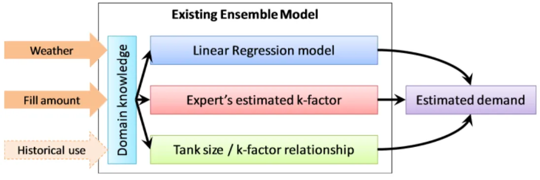
Figure 1.3: Visual representation of the existing model
1.4 Current Process
Currently, the heating oil demand is forecast using an ensemble model. As seen in Figure 1.3, the ensemble model consists of three components: the Linear Regression (LR) model, an expert’s estimated K-factor (measure of the response of use to variations in temperature), and the tank size and K-factor relationship. Additionally, the ensemble model contains other enhancements based on domain knowledge. An estimated demand is calculated by combining the output from these components.
1.4.1 Linear Regression Model
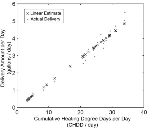
The Linear Regression (LR) model takes advantage of the primarily linear relationship between the heating oil demand and heating degree days. This is demonstrated in Figure 1.4, which plots the Cumulative Heating Degree Day against the delivery amount. Since the LR model is a daily model, we divide the
Cumulative Heating Degree Days and the delivery amount by the number of days between deliveries. The plot clearly shows a linear trend where the delivery amount increases as the weather becomes colder and the cumulative heating degree day increases. The LR model is driven by weather inputs (actual and forecast wind and temperature data) with the following variables:
• sbk is the estimated heating oil demand on thekth day in gallons
• βb0 is the estimated baseload (BL) in gallons
• βb1 is the estimated heatload coefficient in gallons per Heating Degree Day • Kb is the estimated K-factor in Heating Degree Days per gallon
• x1,k or HDD60,k is the Heating Degree Day with reference temperature 60◦F on the kth day
The model itself is expressed as
b
sk=βb0+βb1x1,k =βb0+ (1/Kb)HDD60,k. (1.1)
Baseload describes the portion of the demand that is not affected by the daily average temperature. We expect that space heating does not occur when the temperature is high (i.e. during the summer months). Therefore, baseload for
Figure 1.4: Heating Oil Consumption vs. Heating Degree Days space heating customers theoretically should be zero. However, fitting a regression model often causes the baseload coefficient to be a small non-zero value for space heating customers. The baseload for space and water heating customers is typically a positive value because water heating occurs regardless of the temperature.
Heatload coefficient describes how a customer is “sensitive” to temperature change. Its unit is gallons per Heating Degree Day. A customer with a large heatload coefficient is said to be sensitive to the daily average temperature because a one degree increase in the Heating Degree Day greatly increases the estimated demand.
K-factor is the number of Heating Degree Days required to consume one gallon of heating oil. Its unit is Heating Degree Days per gallon. One can think of this factor as a miles-per-gallon equivalent for a heating oil customer. A large MPG represents a fuel efficient car, and a large K-factor represents a fuel efficient customer. K-factor and the heatload coefficient are inversely related to each other.
Heating Degree Day (HDD) is defined as the reference temperature (Tref) minus the average temperature on the kth day (Tk). If the subtraction results in a negative number (i.e. if the average temperature is greater than the reference temperature), then the HDD is set to 0:
HDDTref,k = max(0, Tref −Tk).
The concept of Heating Degree Day was introduced because of the non-linear relationship between the daily average temperature and the heating oil demand. In other words, Heating Degree Day mathematically expresses the fact that customers no longer consume heating oil when the temperature is warmer than, say, 65◦F.
1.4.2 Expert’s Estimated K-factor
A domain expert at the heating oil company provides his own K-factor estimate for each delivery. This piece of information is especially valuable during the initial deliveries when domain knowledge compensates for the lack of historical data. The weight of this component is reduced as the number of deliveries (and the amount of historical data available) increase.
1.4.3 Tank Size and K-factor Relationship
This component takes advantage of the domain knowledge that customers have large fuel tanks because they tend to consume more fuel. This suggests that the K-factor is inversely proportional to the tank size. Hence we fit a simple linear regression model to the existing customers’ tank sizes and K-factor estimates. The slope and intercept parameter estimates are used to estimate the target customer’s
K-factor based on the customer’s tank size. Similar to the expert’s estimated
K-factor, the weight of this component is reduced as the number of delivery increases.
1.5 Problem with the Current Process
The operation and performance of the ensemble model changes depending on the amount of available historical data. Transient (Figure 1.5) refers to the
start-up period when there is limited historical data. Steady-state (Figure 1.6) refers to a time period when there is enough historical data to perform reliable forecasting.
Figure 1.5: Visual representation of the existing model in its transient state
Figure 1.6: Visual representation of the existing model in its steady state
During the transient period, the ensemble model combines all three
components to compensate for the lack of data. In the steady-state, the ensemble model only uses the LR model. In general, the model’s performance improves as the
amount of available historical data increases. Hence, this method performs well with existing customers who reached steady-state by accumulating large numbers of past deliveries. Since the current method heavily relies on historical data, the method’s forecasting accuracy diminishes for new customers who lack historical data.
1.6 Problem Statement
This thesis addresses the following business and mathematical problem:
• Business statement: To lower the operating costs for a heating oil sales and distribution company by improving new customers’ heating oil demand
forecast for initial deliveries.
• Mathematical statement: Develop a Bayesian forecasting method that reduces the error between the new customers’ forecast and actual heating oil demand during initial deliveries.
The preceding sections provided an overview of the problem and the context of this project. The next two sections focus on the details of the project and the solution: proposed solution, assumptions, and evaluation methods.
1.7 Assumptions
This section outlines the key assumptions of this research project. The summary of each assumption and the reasons why it is necessary are outlined below.
1.7.1 Availability of Historical Data
Target customeris a customer whose future heating oil consumption is
being forecast. Existing customer is a customer whose past forecast and delivery
amount are known to the forecaster at the time of the forecast. This project focuses on cases where there are little to no historical data available for the target
customers. This project, however, assumes that sufficient historical data for
existing customers are available at the time of the forecast. This distinction is important since this research is not about forecasting demand withoutany
historical data, but aboutforecasting demand of the target customer using historical
data from other existing customers.
It should be noted that this approach is similar to surrogate modeling, which
mimics or forecasts the behavior of an original system by constructing a surrogate system using samples taken from the original system [12]. Hence, a surrogate
method can be used to predict the behavior of a surrogate system (target customers) by taking samples (historical data) from the original system (“donor” customers) [7].
1.7.2 Demand Forecast and Actual Use
Since the actual use cannot be measured directly, the actual use is assumed to be the amount delivered during a delivery. This assumption holds well if the tank is always filled to its capacity. However, there are cases when the amount delivered does not equal the actual use. For example, the tank sometimes is not fully refilled because the delivery truck ran out of oil or the shutoff valve prematurely triggered. These special cases are handled by an underfill-overfill detection mechanism.
When the tank is not fully refilled, the amount delivered is likely to be significantly less than the estimated demand. Hence, this is known as an underfill condition. Typically, the company schedules another delivery to finish filling the tank. The amount delivered during this followup delivery is likely to be significantly more than the estimated demand. Hence, this is known as an overfill condition. The detection mechanism detects this condition by checking previous deliveries for each customer. If a customer has an underfill delivery immediately followed by an overfill delivery, then the mechanism replaces the two deliveries with a single artificial delivery computed by adding the delivery amount and heating degree days from the two deliveries.
1.7.3 Stationarity of the K-factor
K-factor describes how fuel efficient a customer is. Unless there is a major change in the behavior of a customer (long vacation away from home, major house renovations that improved insulation, installation of a new furnace, newborn infant in the house, aging parents visiting, etc.), K-factor should remain relatively
constant. This is important for our Bayesian Heating Oil Forecaster because the proposed method is trying to unbias the estimates to match the true K-factor. If the customer’s true K-factor is changing frequently, then the adjustment becomes non-trivial. Although the K-factor for a customer may change over a long period of time (i.e., several years), it is very unlikely to change significantly over a short period of time (i.e., during the first few deliveries). Hence, for the scope of the
thesis, the short-term K-factor is assumed to be stationary.
1.7.4 Positive and Negative Errors
In many forecasting applications, positive and negative errors carry different meanings, consequences, and associated costs. In this thesis, errors are defined as Estimated demand−Actual demand =sbk−sk. Hence, a positive error is reported when the estimated demand is larger than the actual demand. A negative error is reported when the estimated demand is smaller than the actual demand. In the area of heating oil forecasting, positive errors increase the number of unnecessary
deliveries because tanks are considered to have less oil than they actually contain. This can increase the overall operation cost for the company. Negative errors might result in customers running out of oil because the tank is estimated to have more oil than it actually contains. Customers who run out of fuel typically switch supplier, which results in lost revenue for the heating oil company. Since costs associated with
loss of customers are much higher than expected increases in operational costs, the
negative errors are less desirable than positive errors.
The assumptions discussed in this section are applicable at a conceptual level. Mathematical assumptions that apply to the estimation process are discussed in later chapters. The next section discusses the evaluation method used to
determine the effectiveness of our Bayesian Heating Oil Forecaster.
1.8 Evaluation
This section briefly outlines the evaluation method and defines the criteria of an acceptable solution. This project is successful if our Bayesian Heating Oil
Forecaster consistently produces better forecasts compared to the existing method for the same set of initial customers.
The comparison of the current and proposed methods is performed using a backtesting system. The backtesting system performs two sets of ex-post forecasts
and compares the forecasting error of the existing forecasting method against the error of our Bayesian Heating Oil Forecaster. The comparison involves the following five steps as shown in Figure 1.7:
Figure 1.7: Steps of the evaluation method
1. The tester specifies a range of dates to use as a test data set. Simulated forecasts that occur during this date range are used to evaluate and compare the existing forecasting method and our Bayesian Heating Oil Forecaster.
2. The backtesting system identifies new customers that signed up during the dates specified.
3. The backtesting system trains the existing forecasting method and our Bayesian Heating Oil Forecaster using training data set that are available up to the beginning of the test data set.
4. The backtesting system performs ex-post forecast using the existing forecasting method for the customers identified in the previous step. This produces a set of forecasts from the existing method for each of the new customers.
5. The backtesting system performs ex-post forecast using our Bayesian Heating Oil Forecaster for the same set of customers. This produces a set of forecasts from the proposed method for each of the new customers.
6. The backtesting system compares the two sets of forecasts with the actual delivery amount, computes the errors between them, and reports the result. In general, the method with a smaller forecasting error is considered the better method. The error is measured in Root Mean Squared Error (RMSE) and Mean Absolute Percentage Error (MAPE), as well as a weighted error measure which assigns a larger weight to negative errors (potential loss of customers) than positive errors (potential increase in operational costs).
A more thorough discussion of the evaluation process and the backtesting system can be found in Chapter 3. The next section briefly reviews the structure of the remainder of this thesis.
1.9 Organization of this Thesis
This thesis consists of five chapters. Chapter 1 introduced the project background, current process, and the details of the problem being addressed. Chapter 2 provides an overview of the Bayesian forecasting techniques applied to various real-world data sets. Chapter 3 introduces our Bayesian Heating Oil
Forecaster and how it applies to our test data set. Chapter 4 compares the results of our Bayesian Heating Oil Forecaster with those of the existing forecasting method. Finally, Chapter 5 offers conclusions and opportunities for further research.
CHAPTER 2
Survey of Energy Forecasting Literature
Chapter 1 introduced and outlined the problem of forecasting new customers’ heating oil demand. Chapter 2 provides an overview of existing demand forecasting techniques, such as Multiple Linear Regression, Artificial Neural Network, and Ensemble forecasting. Examples of Bayesian forecasting techniques, such as Bayesian Network and Dynamic Linear Model, are discussed. This chapter also contains an overview of the mathematical concepts such as regression analysis and Bayes’ Theorem. These are fundamental concepts used in our Bayesian Heating Oil Forecaster presented in Chapter 3.
2.1 Existing Demand Forecasting Methods
Multiple Linear Regression, Artificial Neural Network, and Ensemble forecasting are three forecasting methods that have been applied successfully to demand forecasting, namely natural gas daily demand forecasting [48]. This section presents an overview of these methods.
2.1.1 Multiple Linear Regression
A multiple linear regression model expresses the dependent variable as a function of one or more independent variables assuming a linear relationship [6; 48]. Suppose we want to forecast a daily demandS on a kth day in the future, using m
independent variables, xk,j, where j = 1, . . . , m. Then the estimated daily demand on the kth day is sk ≈sbk =β0+ m ∑ j=1 βjxk,j ,
where βjs are parameters that describe how independent variables are related to the estimated daily demand. The independent variable xk,1 may represent Heating Degree Days, while β0 is the baseload, and β1 is the heatload coefficient.
Multiple linear regression extrapolates very predictably, adapting well to situations where the inputs are different from past observations. However, multiple linear regression performs poorly when the linearity assumption does not hold. Since past observations are used to estimate the parameters, a multiple linear regression model requires historical data. Generally, the more historical data is available, the better the parameter estimates [48].
A more thorough discussion of the Multiple Linear Regression technique can be found in introductory textbooks such as Forecasting, Time Series, and
Regression: An Applied Approach [6] and Introduction to Linear Regression
Analysis [32].
2.1.2 Artificial Neural Network
Another tool commonly used for estimation and forecasting is an Artificial Neural Network (ANN). An ANN maps an unknown nonlinear relationship between the inputs and the output. This mapping is accomplished through a training
process during which the ANN learns from past observations. Because an ANN handles nonlinear relationships, multiple related factors, such as temperature, wind speed, and prior day temperatures can be used as inputs [48].
An ANN excels when the inputs are similar to, but not the same as, the training data. However, an ANN does not perform as well in cases where the inputs are beyond the domain of the training knowledge. For example, the accuracy of an ANN diminishes when it forecasts natural gas demand for the coldest day on record. Since an ANN must be trained using past observations to expand the domain of the training knowledge, it is not suitable for situations where there is little historical data [48].
A more thorough discussion of Artificial Neural Networks can be found in
Gateway to Memory: An Introduction to Neural Network Modeling of the
Hippocampus and Learning [23].
2.1.3 Ensemble and Combined Forecasts
Ensemble forecasting combines multiple forecasts produced by different forecast methods to obtain a single forecast with variance smaller than the variance of any of the components. Various factors influence dependent variables, and factors that are captured by any one of the forecast methods might be incomplete and limited. However, multiple forecast methods can better capture these factors when combined together. The combined forecast tends to reduce the effects of faulty assumptions, bias, or mistakes in data [2; 48]. As a result, combined forecasts almost unanimously increases forecast accuracy, regardless of the nature of the forecast [9]. Even simple averaging, the most simple combination method, is shown to improve the performance of the forecast [2]. In general, forecasts are combined by taking an weighted average of multiple independent forecasts, or according to a set of rules. Weights are calculated according to a repeatable rule, such as equal weighting, domain knowledge, and past forecast accuracy. Other methods include voting, simulation, combiner, stacked generalization, principle component analysis, singular value decomposition, and artificial neural networks [15]. As specific examples of existing ensemble forecasting techniques, Dhillon cites Fan et al. [17],
whose work introduces and compares combiner and stacked generalization, which are meta-learning techniques that improves the performance of a single classifier by combining multiple classifiers. Ara´ujo and New [1] apply ensemble forecasting frameworks, such as the bounding box, consensus, and probabilistic techniques, to improve the robustness of bioclimatic modeling.
Readers who are interested in additional materials should also refer to an annotated bibliography by Clemen [9]. Clemen offers a brief overview, historical development, and an extensive list of over 200 applied and theoretical articles covering various combined forecasting techniques.
This concludes the brief overview of the existing forecasting techniques used in energy demand forecasting. The following section discusses the Bayesian
approach to probability and forecasting.
2.2 Bayes’ Theorem, Bayesian Probability, and Bayesian Inference
Various Bayesian techniques discussed in the remainder of this thesis, including our Bayesian Heating Oil Forecaster, take advantage of the Bayesian approach to forecasting. This section provides an introduction to Bayes’ Theorem to gain a better understanding of the Bayesian approach to forecasting, and how various Bayesian forecasting techniques are implemented. Materials and discussions
contained in this and later sections are drawn from textbooks on Bayesian
forecasting such asIntroduction to Bayesian Statistics [5] andStatistics: A Bayesian
Perspective [4]. Both are introductory statistics textbooks that extensively use
Bayesian inference. The latter book is recommended especially for readers interested in a solid review of probability theory. Introduction to Bayesian Statistics [5] is for
upper level undergraduate students with a background in calculus and probability theory. It offers in-depth discussions of Bayesian probability and statistics.
Bayes’ Theorem was proposed by Reverend Thomas Bayes in the 18th century and was later extended by Laplace in the 19th century [36; 47]. From a statistical inference perspective, the theorem is significant because it allows one to infer the probability of a cause when its effect is observed [36]. In other words, Bayes’ Theorem helps answer questions such as “I have a stiff neck (effect). How likely am I to have a meningitis (cause)?”, see Figure 2.1.
Figure 2.1: How likely is a cause given the effect? [33]
in which the probabilities change in the light of evidence [4]. In other words, Bayes’ Theorem describes mathematically the process by which forecasters update their knowledge in response to an observed event, as suggested by Figure 2.2.
Figure 2.2: A model of how Bayes’ Theorem updates forecaster knowledge
The knowledge of the forecaster is represented mathematically using
probability distributions. The update process can be described using three distinct probability distributions:
Prior represents our knowledge before we observe evidence. The prior probability of an event A is expressed as P(A).
Likelihood represents a factor that is used to update our prior knowledge. The likelihood for an eventA and an evidence B is expressed in terms of a conditional probabilityP(B|A).
probability of an eventA given the evidence B is expressed in terms of a conditional probabilityP(A|B).
In summary, Bayes’ Theorem says
P(A|B) = P(B|A)P(A)
P(B) .
It states that the posterior is proportional to the product of the prior and the likelihood. In other words, we can obtain our posterior knowledge by 1) multiplying our prior and the likelihood and 2) scaling the product.
Figure 2.2 graphically represents how the forecasters update their knowledge using the prior, likelihood, and posterior distributions. As seen in the diagram, the update process is iterative: The current posterior becomes the prior of the next step. The process iterates when a new event is observed.
The following two sections further describe Bayes’ Theorem using simple examples. The first section describes the theorem using discrete probability distributions. The second section describes the theorem using continuous probability distributions.
2.2.1 Discrete Bayesian Analysis
This section applies Bayes’ Theorem using two separate examples. The first example is a very simple balls-in-an-urn example drawn from Bolstad [5]. This example illustrates how the prior, likelihood, and posterior distributions interact to update the forecaster’s knowledge about a model. The second example involves forecasting the relative strength of two basketball teams. The basketball example, drawn from Berry [4], illustrates how to apply Bayes’ Theorem to perform forecasts. Later, the second example is extended to illustrate the difference between discrete and continuous Bayesian forecasting.
Example: Balls-in-an-urn
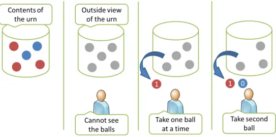
Suppose there is an urn with five balls inside. The balls are colored either red or blue, but we cannot see the contents of the urn. The objective is to estimate the number of red balls in the urn by drawing a ball out of the urn one by one without replacement. Since we are interested in the number of red balls, let the random variable X be the number of red balls in the urn. If we draw a ball from the urn, the color of the ball is either red or blue. To represent this mathematically, let the random variableY = 1 if the draw is red, andY = 0 if the draw is blue.
Figure 2.3: The balls-in-an-urn example
Prior and posterior beliefs
As stated above, our objective is to estimate the number of red balls in the urn. Hence, our belief is our estimate of the number of red balls in the urn. Our prior belief is our estimate of the number of red balls in the urn before we draw a
ball. Our posterior belief is our estimate of the number of red balls in the urn after
we draw a ball. Note that our prior and posterior beliefs change as we continue to draw the balls out of the urn. For example, our first prior belief (denoted Prior(1))
is our estimate of the number of red balls in the urn before we draw the first
ball out of the urn. Our first posterior belief (denoted Posterior(1)) is our estimate
of the number of red balls in the urnafter we draw the first ball out of the urn.
Posterior(1) is also our Prior(2) because Posterior(1) is our estimate before we draw
can be summarized as
Posterior(n) = Prior(n+ 1) for n≥1.
First prior belief
Although Prior(n) for n≥2 are computed iteratively, we have to present our own estimate for Prior(1). Initially, we know that the total number of balls in the urn is five, but we have no idea how many of them are red. What we know for sure is that the number of red balls can be only 0, 1, 2, 3, 4, or 5. In this case, we might assume that all possible outcomes are equally likely. Translating this prior
knowledge into probability gives
P(X = 0) =P(X = 1) =...=P(X = 5) = 1/6, and
P(X <0) =P(X >5) = 0.
Likelihood
Likelihood is the probability of observing an evidence given the truth. The “evidence” is the color of the ball we draw from the urn. The “truth” is the actual number of red balls in the urn. In other words, it describes how “likely” it is to draw a ball with a certain color if the number of red balls in the urn is either 0, 1, 2, 3, 4, or 5. For instance, P(Y = 1|X = 2) represents the likelihood (probability) of
drawing a red ball from the urn if the number of red balls in the urn is 2. Since there are 5 balls in the urn, the likelihood of drawing a red ball from the urn when there are 2 red balls in the urn is 2 out of 5. Using the notation for conditional probability, this can be written as
P( draw red ball |number of red ball in the urn = 2) = P(Y = 1|X = 2) = 2/5.
The likelihood changes as the observation (the color of the ball drawn) changes. For example, P(Y = 0|X = 2) represents the likelihood (probability) of drawing a blue ball from the urn if the number of red balls in the urn is 2. Since there are a total of 5 balls, if there are 2 red balls, then the remaining 3 would be blue. Hence,
P( draw blue ball |number of red ball in the urn = 2) =P(Y = 0|X = 2) = 3/5.
Update Using Joint Probability
In this example, we have two different random variables,
X = number of red balls in the urn, and Y = color of the ball. The probability that
X =xi and Y =yi occur simultaneously is called the joint probability,
f(xi, yi) =P(X =xi, Y =yi).
draw a red ball occurring simultaneously is expressed as f(2,1) =P(X = 2, Y = 1).
Since we have a total of 5 balls and 2 colors, there are 10 possible joint probabilities. The 10 joint probabilities together form ajoint probability distribution of the random variables X and Y. A joint probability distribution represents the
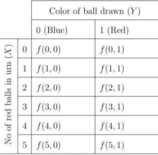
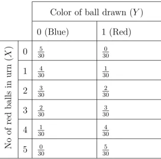
probability of all possible combinations of the joint random variables, and can be expressed in a table form as shown in Table 2.1.
Color of ball drawn (Y)
0 (Blue) 1 (Red) No of red balls in urn ( X ) 0 f(0,0) f(0,1) 1 f(1,0) f(1,1) 2 f(2,0) f(2,1) 3 f(3,0) f(3,1) 4 f(4,0) f(4,1) 5 f(5,0) f(5,1)
Table 2.1: Joint probability distribution for the balls-in-an-urn example
Individual joint probability can be computed using the following relationship:
f(xi, yi) = g(xi)×f(yi|xi), and (2.1)
P(X =xi∧Y =yi) = P(X =xi)×P(Y =yi|X =xi). (2.2)
Since we update our prior belief by multiplying our prior belief and an appropriate likelihood, calculating the joint probability is equivalent to updating our prior belief
using an appropriate likelihood. The joint probabilities for the case when the first ball picked is red can be computed as follows:
f(0,1) =P(X = 0)×P(Y = 1|X = 0) = 1/6×0/5 = 0 f(1,1) =P(X = 1)×P(Y = 1|X = 1) = 1/6×1/5 = 1/30 f(2,1) =P(X = 2)×P(Y = 1|X = 2) = 1/6×2/5 = 2/30 f(3,1) =P(X = 3)×P(Y = 1|X = 3) = 1/6×3/5 = 3/30 f(4,1) =P(X = 4)×P(Y = 1|X = 4) = 1/6×4/5 = 4/30 f(5,1) =P(X = 5)×P(Y = 1|X = 5) = 1/6×5/5 = 5/30.
If we repeat the calculation for the case when the ball is blue, then we can obtain a full joint probability distribution as shown in Table 2.2.
Color of ball drawn (Y)
0 (Blue) 1 (Red) No of red balls in urn ( X ) 0 305 300 1 4 30 1 30 2 303 302 3 302 303 4 301 304 5 0 30 5 30
Table 2.2: Joint probability distribution for the balls-in-an-urn example with joint probabilities calculated
If the first ball was red, then the column in the joint probability distribution with Y = 1 is our posterior knowledge, except that the sum of the products of the priors and the likelihoods equal to 1/2. Since our knowledge must be expressed in terms of probability, the sum must equal to 1. This can be accomplished by dividing (scaling) the products by the sum of the products.
Repeat
As we repeat the drawings, we also repeat the calculations. For the second draw, the posterior we obtained after the first draw becomes our new prior. The update process continues as we draw more balls from the urn. The actual
calculations are shown in Tables 2.3 and 2.4. The posterior probability in Table 2.3 replicates the above calculation and shows the case when the first ball drawn is red. The posterior probability in Table 2.3 is when the second ball drawn is blue.
xi (No. of red) Prior Likelihood Prior × Likelihood Posterior
0 1 6 0 5 1 6 × 0 5 = 0 0/ 1 2 = 0 1 16 15 16 ×15 = 301 301/12 = 151 2 16 25 16 ×25 = 302 302/12 = 152 3 16 35 16 ×35 = 303 303/12 = 153 4 16 45 16 ×45 = 304 304/12 = 154 5 16 55 16 ×55 = 305 305/12 = 155 Sum 1 12 1
Table 2.3: Posterior probability distribution after the first observation
xi (No. of red) Prior Likelihood Prior × Likelihood Posterior 0 0 0 1 151 44 151 × 44 = 151 151/13 = 102 2 152 34 152 × 34 = 101 101/13 = 103 3 153 24 153 × 24 = 101 101/13 = 103 4 154 14 154 × 14 = 151 151/13 = 102 5 155 0 155 ×0 = 0 0/13 = 0 Sum 1 13 1
Table 2.4: Posterior probability distribution after the second observation likelihood, and posterior belief. The update process illustrates how Bayesian inference is applied to estimate the probability of an unknown and unobservable quantity (number of red balls in the urn) in light of evidence (the color of the ball that is drawn from the urn). The next example focuses more on how to apply Bayesian inference in the context of forecasting.
Example: Relative strength of two basketball teams
This example is adapted from a similar example presented by Berry [4]. Consider two basketball teams: MU and UC. The two teams belong to the same conference, and have several games each season. Our objective is to estimate the relative strength of MU, and forecast the probability of MU winning the next game
against UC. A relative strength of 0 means MU can never win over UC. A relative strength of 1 means MU can always win over UC. If the relative strength is 0.8, then
MU is expected to win over UC for 80 percent of the time. Suppose the season just started so that the two teams have not met this season. Since we are interested in the relative strength of MU, let the random variable X be the relative strength of MU. To simplify the problem, let us also assume that the teams will either win or lose and will never end a game with a tie. To represent this mathematically, let the
random variable Y = 1 if MU wins, and Y = 0 if UC wins. Figure 2.4 summarizes
this setup.
Figure 2.4: Relative strength of basketball teams example
Prior and posterior beliefs
Our objective in this example is to estimate the relative strength of MU by observing games between MU and UC so that we can forecast the winner of the next game. Hence, our belief is our estimate of the relative strength of MU. Using the same notation presented in the balls-in-an-urn example, our prior belief,
Prior(n), is our estimate of the relative strength of MUbefore we observe thenth
game of the current season. Our posterior belief, Posterior(n), is our estimate of the relative strength of MU after we observe the nth game.
First prior belief
Next, we have to present our own estimate for Prior(1). Initially we know that the relative strength can range between 0 and 1. To simplify the example, we discretize the range by 0.1 increments so that the only possible relative strengths are 0.0, 0.1, 0.2, 0.3, 0.4, 0.5, 0.6, 0.7, 0.8, 0.9, and 1.0. Additionally, say we are informed that MU was stronger than UC during last year’s season, but both teams won at least once during the same period. It seems reasonable to assume that relative strengths of 0.0 and 1.0 are unlikely, and relative strengths greater than 0.5 are more probable than relative strengths less than 0.5. Translating this prior knowledge into probability might look like Table 2.5:
Strength of MU 0.0 0.1 0.2 0.3 0.4 0.5 0.6 0.7 0.8 0.9 1.0 Sum
Probability 0% 2% 3% 5% 8% 12% 22% 26% 17% 5% 0% 100%
Strength×Probability 0.00 0.00 0.01 0.02 0.03 0.06 0.13 0.18 0.14 0.05 0.00 0.61
Table 2.5: An example of a possible Prior(1) for the basketball example
Notice that unlike our first example, we have assigned unequal probabilities to different strengths. These probabilities can be our best guess, since the update process adjusts these estimates based on future observations. Our objective is to forecast the winner of the next game. This can be accomplished by computing the
predicted relative strength of MU. The predicted relative strength of MU is computed by multiplying each of the possible relative strengths of MU by its probability and adding the products. The figure shows that the predicted relative strength of MU is 0.61. This matches our expectation since we assumed that MU might continue to be stronger than UC during the current season.
Likelihood
Likelihood is the probability of observing an evidence given the truth. The “evidence” is the result of the game. The “truth” is the actual relative strength of MU. In other words, it describes how “likely” it is for MU to win if the actual relative strength of MU is either 0, 0.1, 0.2, ..., 0.9, or 1.0. For instance,
P(Y = 1|X = 0.2) represents the likelihood (probability) of MU winning the game if the relative strength of MU is 0.2. If the relative strength of MU is 0.2, then the likelihood of MU winning the game is also 0.2. Using the notation for conditional probability, this can be written as
Likelihood =P( MU wins | actual relative strength of MU = 0.2)
=P(Y = 1|X= 0.2) = 0.2.
MU losing the game if its actual relative strength is 0.2 is
Likelihood =P( MU loses |actual relative strength of MU = 0.2) =P(Y = 0|X = 0.2)
= 1−0.2 = 0.8.
Table 2.6 shows two different likelihoods for all possible relative strengths (0.0, 0.1, ..., 1.0; columns in the figure) and for all possible outcomes (MU wins, MU loses; rows in the figure).
Strength of MU 0.0 0.1 0.2 0.3 0.4 0.5 0.6 0.7 0.8 0.9 1.0
Likelihood of MU winning 0.0 0.1 0.2 0.3 0.4 0.5 0.6 0.7 0.8 0.9 1.0 Likelihood of MU losing 1.0 0.9 0.8 0.7 0.6 0.5 0.4 0.3 0.2 0.1 0.0
Table 2.6: Likelihood for the basketball example
Update
multiplying our prior belief and the likelihood: P(X = 0.0)×P(Y = 1|X = 0.0) = 0.0×0.0 = 0 P(X = 0.1)×P(Y = 1|X = 0.1) = 0.02×0.1 = 0.002 ... P(X = 0.9)×P(Y = 1|X = 0.9) = 0.05×0.9 = 0.045 P(X = 1.0)×P(Y = 1|X = 1.0) = 0.0×1.0 = 0.
Table 2.7 shows the update calculation for all possible relative strengths (0.0, 0.1, ..., 1.0; columns in the figure). The posterior row is computed by dividing (scaling) the products by the sum.
Model 1 2 3 4 5 6 7 8 9 10 11 Sum
Strength 0.0 0.1 0.2 0.3 0.4 0.5 0.6 0.7 0.8 0.9 1.0
-Prior 0% 2% 3% 5% 8% 12% 22% 26% 17% 5% 0% 100%
Likelihood (MU wins) 0.0 0.1 0.2 0.3 0.4 0.5 0.6 0.7 0.8 0.9 1.0
-Prior×Likelihood 0.000 0.002 0.006 0.015 0.032 0.060 0.132 0.182 0.136 0.045 0.000 0.61
Posterior 0.0% 0.3% 1.0% 2.5% 5.2% 9.8% 21.6% 29.8% 22.3% 7.4% 0.0% 100%
Strength×Posterior 0.000 0.000 0.002 0.007 0.021 0.049 0.130 0.209 0.178 0.066 0.000 0.66
Table 2.7: Update for the basketball example
The posterior belief is our estimate of the relative strength of MU after the first game. The predicted relative strength of MU after the first game is computed by multiplying each of the possible relative strengths of MU by its probability and adding the products. Table 2.7 shows that the predicted relative strength of MU is
0.66, which is larger than the initial estimate of 0.61. This matches our expectation since MU just won the first game.
This example illustrates the application of Bayesian inference to estimate the probability of an unknown and unobservable quantity (relative strength of MU) in light of evidence (results of the game). If we generalize this to energy (heating oil) demand forecasting, Bayesian inference can be used to estimate the probability of an unknown and unobservable quantity (K-factor) in light of evidence (K-factor that is observed between deliveries). Once the K-factor is known, the heating oil demand can be computed using a regression model.
Since the K-factor is a continuous quantity, the next section discusses the difference between the discrete and continuous approaches to Bayesian inference.
2.2.2 Continuous Bayes Inference
The logical steps of computing the continuous Bayesian inference is identical to its discrete counterpart: we start with a prior belief, observe an event, update our belief, and compute the posterior belief. What differs between the two are the use of continuous random variables and probability distributions.
The balls-in-an-urn example is a discrete example since the quantity (number of balls; 1,2,3,4,5) as well as the possible outcomes (red/blue) are discrete. The
basketball example has a continuous quantity (relative strength; ranging from (0...1)) and discrete outcomes (win/lose). Any continuous probability distribution can be used to describe the continues random variable, including but are not limited to uniform, beta, gamma, normal, and empirical distributions [5].
Empirical Distribution
An empirical distribution is a probability distribution that is generated directly from the observed (sample) data. It represents the estimated probability of a certain observation occurring in the population. A histogram is a scaled version of the empirical probability density function. An empirical PDF is computed by
scaling the histogram: count
sample size×bin width.
Beta Distribution
A beta distribution frequently is used in the context of Bayesian estimation because it drastically simplifies the update process [4; 5]. A beta distribution is parameterized by two parameters, often denoted bya and b. The distribution itself is sometimes denoted as β(a, b). The probability function of the beta distribution
β(a, b) is P(x) =f(x;a, b) = 1 B(a, b)x a−1(1−x)b−1 = (a+b−1)! (a−1)!(b−1)!x a−1(1−x)b−1.
Beta distributions have the following properties that help simplify the update process [4; 5]:
• The product of two beta distributions is a beta distribution, and
• Multiplication of two beta distributions can be accomplished by adding their parameter values.
The above properties are demonstrated below:
f(x;a1, b1)×f(x;a2, b2) = 1 B(a1, b1)B(a2, b2) x(a1−1)(1−x)(b1−1)x(a2−1)(1−x)(b2−1) = 1 B(a1+a2−2, b1+b2−2) x(a1+a2−2)(1−x)(b1+b2−2) =f(x;a1+a2−2, b1+b2−2).
The expected value of a beta distribution is computed from the parameter values,
E(X) = a
Maximum Likelihood Estimation
We use distribution fitting techniques, such as maximum likelihood estimation (MLE), to fit a continuous distribution to a set of data. Maximum likelihood estimation is a statistical technique that identifies a probability
distribution that makes the observed data most likely. In other words, it maximizes the likelihood P( observed data | parameters ) for a set of probability distribution parameters and observed data. Since each probability distribution is different, the maximum likelihood estimation for each distribution is also different.
The maximum likelihood estimates for the Beta distribution are computed numerically based on the equation given by Johnson, Kotz, and Balakrishnan [29]. Others, such as Beckman and Tietjen [3] have developed a numerical technique in which the maximum likelihood estimates for the Beta parameters are computed.
Readers who are interested in an introduction to maximum likelihood estimates may read an article by Myung for a quick introduction [35]. Moore [34] uses a Gaussian distribution to step through the calculation process of maximum likelihood estimation. The NIST handbook also has an entry about likelihood estimation for Beta distributions [19].
2.3 Existing Bayesian Forecasting Methods
Bayesian forecasting methods have unique advantages over traditional
forecasting methods. One advantage is their effectiveness during the initial transient period when little or no prior data is available [28]. This section provides an
overview of Bayesian forecasting techniques that have been applied in areas including engineering, business, meteorology, and energy. This should help us see how the Bayesian forecasting algorithm, presented in Chapter 3, is related to other techniques that are already in use.
2.3.1 Bayesian Networks
A Bayesian Network is a probabilistic graphical model that often drastically reduces the computational complexity of the original problem [33]. The network is a graphical representation of the probabilistic relationships among many variables with cause-effect relationships [36]. The nodes in the network represent random variables, and edges represent dependence among the variables. A network as a whole represents a joint probability distribution over a set of random variables. In other words, the network represents all possible combinations of the joint random variables and their probabilities. It is a directed acyclic graph: each node is guaranteed not to be its own child or its own parent (Figure 2.5).
Figure 2.5: Example Bayesian network modeling causes of wet grass [45] Each variable is only dependent on its parents, which means that they are independent from all other non-parent variables. This independence frequently enables the model to reduce the number of parameters compared to the model that does not account for such independence. It also drastically simplifies the joint probability distribution. Simplifying the joint probability distributions reduces the cost of computing the posterior probabilities. For cases where the joint probability distribution is large, the calculation becomes impractical without simplifying the joint probability distribution using a Bayesian Network [36; 43].
To illustrate how a Bayesian Network can be constructed and used, let us consider the following simple example adopted from a lecture by Moore [33]. You are at a small regional airport interested in estimating the probability of delays under various conditions. Suppose we have the following five events:
• S: It is sunny.
• M: The airline is Delta. (If not, then it is United.)
• R: The airplane is Boeing. (If not, it is Airbus.)
• L: The airplane arrives late.
• T: The airplane leaves on time.
Figure 2.6: Example joint probability distribution [33]
Figure 2.6 is an example of a joint probability distribution that expresses the uncertainty involved in this problem. The joint probability distribution can be used to calculate various probabilities such as
• the probability that the airplane leaves on time, when it is raining (S = 0), the airline is Delta (M = 1), the airplane is Boeing (R = 1), and the airplane
arrives on time (L= 0):
P(T|¬S∧M ∧R∧ ¬L);
• the probability that the airplane leaves on time, when the airline is United and it is sunny:
P(T|¬M ∧S);
• the probability that the airplane arrives late, when the airplane is Airbus:
P(L|¬R).
Specifying the entire joint probability distribution with five binary random variables requires 32 different probabilities. The following example uses the
Bayesian Network to reduce the number of probabilities required to calculate the joint probability distribution from 32 to 10.
A Bayesian Network requires knowledge of the cause-effect relationships among the five variables. For this example, the following assumptions are made:
• Weather condition does not depend on and does not influence which airline is
• Weather condition does not depend on and does not influence the manufacturer of the aircraft.
• Once we know which airline is flying the aircraft, then whether it arrives late does not affect the manufacturer of the aircraft.
• Regardless of the airline, flights are frequently delayed due to bad weather.
• United is more likely to arrive late than Delta.
• United is more likely to use Boeing aircraft than Delta.
• Airplanes are more likely to leave on time if the airplanes arrived on time.
The first assumption describes the independence between weather condition and the airline. This is specified by the statement P(S|M) =P(S). Similarly, the second assumption describes the independence between the weather condition and the aircraft manufacturer. This is specified by the statement P(S|R) =P(S). The third assumption is a conditional independence between airplane manufacturer and the lateness of the flight given the airline. In other words, L and R are conditionally independent given M. This is specified by the statement P(L|M, R) =P(L|M) and
P(R|M, L) =P(R|M). The fourth assumption indicates that weather condition influences the lateness of the flight. The fifth assumption indicates that the airline influences the lateness of the flight. Similarly, the sixth assumption indicates that the airline influences which manufacturer built the aircraft. The last assumption
indicates that arriving late influences the probability of leaving on time. Expressing these assumptions using a Bayesian Network, we obtain Figure 2.7.
Figure 2.7: An example Bayesian Network that describes flight delays [33]
We used known relationships among variables to construct the Bayesian Network. The next step is to assign probabilities that describe each node. In general, the table for node A must list P(a|Parent values) for each possible
combination of parent values. For example, node L is dependent on parents S and
M. Hence, possible combinations are:
• P(L|M ∧S) =P(Airplane arrives late|Airline is Delta∧Sunny)
• P(L|M ∧ ¬S) =P(Airplane arrives late|Airline is Delta∧Rainy)
• P(L|¬M ∧S) =P(Airplane arrives late|Airline is United∧Sunny)
• P(L|¬M ∧ ¬S) =P(Airplane arrives late|Airline is United∧Rainy)
observations, or experiments. Suppose we reviewed the on-time performance log published by the airport and empirically determined the probabilities:
• When the airline was Delta and it wassunny, the flight arrived late 5% of the time =P(L|M ∧S) = 0.05.
• When the airline was Delta and it wasrainy, the flight arrived late 10% of the time =P(L|M ∧ ¬S) = 0.1.
• When the airline was United and it wassunny, the flight arrived late 10% of the time = P(L|¬M ∧S) = 0.1.
• When the airline was United and it wasrainy, the flight arrived late 20% of the time = P(L|¬M ∧ ¬S) = 0.2. Hence, • P(¬L|M ∧S) = 1−0.05 = 0.95, • P(¬L|M ∧ ¬S) = 1−0.1 = 0.9, • P(¬L|¬M ∧S) = 1−0.1 = 0.9, and • P(¬L|¬M ∧ ¬S) = 1−0.2 = 0.8.
Repeating this for all nodes in the graph, we obtain Figure 2.8 with 10 probabilities:

![Figure 2.5: Example Bayesian network modeling causes of wet grass [45]](https://thumb-us.123doks.com/thumbv2/123dok_us/493795.2558421/55.918.295.680.112.427/figure-example-bayesian-network-modeling-causes-wet-grass.webp)
![Figure 2.8: An example Bayesian Network with probabilities [33]](https://thumb-us.123doks.com/thumbv2/123dok_us/493795.2558421/61.918.218.765.105.319/figure-example-bayesian-network-probabilities.webp)

![Figure 2.10: Illustration of nonstationary time series with four pattern regimes [2]](https://thumb-us.123doks.com/thumbv2/123dok_us/493795.2558421/67.918.210.774.118.429/figure-illustration-nonstationary-time-series-pattern-regimes.webp)
