Available at:
http://hdl.handle.net/2078.1/165076
[Downloaded 2019/04/19 at 02:58:01 ]
Paul, Jérôme
Abstract
Modern personalised medicine uses high dimensional genomic data to perform customised diagnostic/prognostic. In addition, physicians record several medical parameters to evaluate some clinical status. In this thesis we are interested in jointly using those different but complementary kinds of variables to perform classification tasks. Our main goal is to provide interpretability to predictive models by reducing the number of used variables to keep only the most relevant ones. Selecting a few variables that allow us to predict some clinical outcome greatly helps medical doctors to understand the studied biological process better. Mixing gene expression data and clinical variables is challenging because of their different nature. Indeed genomic measurements are expressed on a continuous scale while clinical variables can be continuous or categorical. While the biomedical domain is the original incentive to this work, we tackle the more general problem of feature selection in the presen...
Document type : Thèse (Dissertation)
Référence bibliographique
Universit´e catholique de Louvain
Institute of Information and Communication Tech-nologies, Electronics and Applied Mathematics Machine Learning Group
Feature Selection from
Heterogeneous Biomedical Data
—
Providing interpretable models
for high dimensional data
J´erˆome
Paul
Thesis presented for the Ph.D. degree in Engineering Sciences
Thesis jury :
Prof. Pierre Dupont(Universit´e catholique de Louvain), Advisor Prof. Daniel Hern´andez-Lobato(Universidad Aut´onoma de Madrid) Prof. John Lee(Universit´e catholique de Louvain)
Prof. Charles Pecheur(Universit´e catholique de Louvain), Chairman Prof. Yvan Saeys(Universiteit Gent)
Prof. Michel Verleysen(Universit´e catholique de Louvain)
Abstract
Modern personalised medicine uses high dimensional genomic data to perform customised diagnostic/prognostic. In addition, physicians re-cord several medical parameters to evaluate some clinical status. In this thesis we are interested in jointly using those different but complemen-tary kinds of variables to perform classification tasks. Our main goal is to provide interpretability to predictive models by reducing the number of used variables to keep only the most relevant ones. Selecting a few variables that allow us to predict some clinical outcome greatly helps medical doctors to understand the studied biological process better.
Mixing gene expression data and clinical variables is challenging be-cause of their different nature. Indeed genomic measurements are ex-pressed on a continuous scale while clinical variables can be continuous or categorical. While the biomedical domain is the original incentive to this work, we tackle the more general problem of feature selection in the presence of heterogeneous variables. Few variable selection methods jointly handle both kinds of features directly. That is why we focus on tree ensemble methods and kernel approaches.
Tree ensemble methods, like random forests, successfully perform classification from data with heterogeneous variables. In addition, they propose a feature importance index that can rank variables according to their importance in the predictive model. Yet, that index suffers from two main drawbacks. Firstly, the provided feature rankings are highly sensitive to small variations of the datasets. Secondly, while the variables are accurately ranked, it is very difficult to decide which features actually play a role in the decision process. This work puts forward solutions to those two problems. We show in an analysis of tree ensemble methods stabilities that feature rankings get considerably stabler by growing more trees than needed to obtain good predictive performances. We also introduce a statistically interpretable feature selection index. It assesses
whether the variables are important in predicting the class of unseen samples. The output p-values offer a very natural threshold to decide which features are significant.
Apart from tree ensemble approaches, there are few feature selection methods that handle continuous and categorical variables in an embed-ded way. It is however possible to build classifiers that profit from both kinds of data by using kernels. In this thesis, we adapt those techniques to perform heterogeneous feature selection. We propose two kernel-based algorithms that rely on a recursive feature elimination procedure. The importance of the variables is extracted either from a non-linear SVM or multiple kernel learning. Those approaches are shown to provide state-of-the-art results in terms of predictive performances and feature selection stability.
Acknowledgements
Another quest will start from here. You’ll see these words appear on a black screen if you manage to finish ‘The Legend of Zelda’. As I reach the end of my 5-year quest, I would like to thank the people that helped me over this adventure.
Tout d’abord, merci, Pierre, de m’avoir accueilli dans ton ´equipe de recherche. J’ai beaucoup appr´eci´e ces 5 ann´ees sous ta supervision et ton conseil. Nos nombreuses discussions et tes pr´ecieux avis ont forg´e cette th`ese. Je pense et j’esp`ere que tes qualit´es ont un peu d´eteint sur moi, en particulier la rigueur scientifique et le souci du d´etail (le goˆut pour les bonnes bi`eres, je l’avais d´ej`a).
I also would like to thank all the members of my thesis committee and jury. Your questions and remarks helped me a lot improve this work. Special thanks go to Michel for your advices and guidance in the
first years of my thesis and to John for the thorough feedback on the preliminary version of this manuscript.
Je voudrais ´egalement remercier mes coll`egues d’INGI et du Ma-chine Learning Group. Sam, faire notre m´emoire ensemble ´etait d´ej`a tr`es chouette, mais travailler dans le mˆeme bureau, pouvoir discuter de nos sujets respectifs et de plein d’autres choses pendant ces 5 derni`eres ann´ees, c’´etait vraiment g´enial. Merci aussi, Adrien, de nous avoir re-joint dans ces discussions. Il y avait quand mˆeme une sacr´ee ambiance dans ce bureau :-). My thanks also go to my other colleagues of the MLG: Alexandra, Benoit, Dimitri, Emilie, Guillaume, Roberto. Our seminars and discussions were much enjoyable, as well as our trips to Bruges for the ESANN conference. I also thank all the people in INGI. It’s been a very nice working environment.
Je remercie ´egalement mes potes geeks de LLN: Antoine, Fw´e, GBB, JB, JC, Ka, Minou, Nico, Sam, Simon, Xa. On en a fait du chemin depuis ces longues journ´ees `a r´ediger nos m´emoires ensemble en salle
Sun ! Toutes ces bi`eres partag´ees, ces soir´ees, ces discussions et ces mails ´echang´es ont ´et´e pour moi un solide appui pendant cette th`ese. Merci `a mes anciens et actuels colocs — JB et S, Xa, Læti, Jess et Ka — pour cette tr`es chouette ambiance `a l’appart. On en a bien besoin apr`es un gros rush pour soumettre un papier `a temps.
Merci aussi `a mes amis musiciens. Les r´ep´etitions et concerts avec le Quantess Combo’s, Jack Gondry and his New Music, les Blue Caps et le CMN sont des moments pr´ecieux qui me permettent de m’´evader compl`etement. Les troisi`emes mi-temps en votre compagnie sont tout aussi appr´eciables !
Enfin, je voudrais remercier ma famille qui a toujours cru en moi et m’a support´e tout au long du chemin. Merci `a mes parents, Luc et Anne-Fran¸coise. Depuis que je suis tout petit, vous avez ´eveill´e ma curiosit´e et m’avez soutenu dans mes activit´es scolaires, musicales et dans bien d’autres choses. Une bonne partie de cette th`ese vous revient donc aussi ! Merci `a mon fr`ere, Guillaume, et ma sœur, Marie-Aline, de m’avoir soutenu et demand´e de temps en temps, mais pas trop souvent, comment avan¸cait ma recherche. Je pense ´egalement `a ma grand-m`ere, Agn`es, qui me posait r´eguli`erement la question et qui n’est plus l`a pour voir le r´esultat.
For me, it is now time to press the start button again. Thank you all for accompanying me.
Contents
1 Introduction 1
1.1 Machine learning . . . 1
1.2 Heterogeneous biomedical data . . . 2
1.3 Feature selection: what and why ? . . . 4
1.4 What is a good feature selection method ? . . . 5
1.5 Thesis focus . . . 6
1.5.1 Tree ensembles: better feature selection . . . 7
1.5.2 Kernel methods: new feature selection schemes . . 7
1.6 Summary of the contributions . . . 8
1.7 Publication list . . . 9
1.8 Roadmap . . . 9
I Background and materials 11 2 Classification 13 2.1 Definition and notations . . . 14
2.2 Tree ensemble methods . . . 15
2.2.1 Decision trees . . . 15
2.2.2 Ensemble of trees . . . 24
2.2.3 Limitations of approaches based on decision trees 28 2.3 Support vector machines . . . 29
2.3.1 Linear SVM . . . 29
2.3.2 Non-linear classification with the kernel trick . . . 33
2.3.3 Soft-margin SVM . . . 36
2.4 Multiple kernel learning . . . 37
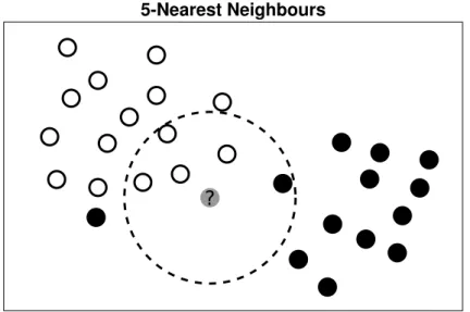
2.5 Instance-based and prototype-based classifiers . . . 39
2.6 Naive Bayes . . . 41
3 Feature selection 45
3.1 Dimensionality reduction . . . 45
3.2 Feature selection paradigms . . . 46
3.2.1 Filters . . . 47
3.2.2 Wrappers . . . 47
3.2.3 Embedded methods . . . 48
3.3 Heterogeneous feature selection . . . 50
3.3.1 Naive approach . . . 50
3.3.2 Wrapping heterogeneous classifiers . . . 51
3.3.3 Variable importance from Random Forest . . . 52
3.3.4 Hybrid feature selection . . . 53
3.3.5 Recursive feature elimination . . . 56
3.4 Extracting statistically significant features from rankings 57 3.4.1 mr-Test . . . 57
3.4.2 1Probe . . . 58
4 Experimental setting 59 4.1 Predictive performances . . . 59
4.2 Feature selection stability . . . 60
4.3 Experimental protocol . . . 61
II More interpretable heterogeneous feature selection methods 65 5 Stable variable rankings from Random Forest 69 5.1 Predictive performances . . . 70
5.2 Stability of class prediction . . . 70
5.3 Stability of feature selection . . . 72
5.4 Conslusion . . . 73
6 Jχ2: A statistically interpretable importance index from Random Forest 75 6.1 Definition of Jχ2 . . . 76
6.2 Concordance withJa . . . 78
6.3 Jχ2 highlights important variables . . . 80
6.4 Good prediction from significant features . . . 82
6.5 Jχ2 outperforms alternatives . . . 82
6.6 Discussion . . . 83
Contents vii 7 Two kernel approaches for heterogeneous feature
selec-tion 85
7.1 IntroducingRF EM KLand RF ESV M . . . 85
7.2 Performance assessment . . . 87
7.3 Conclusion . . . 88
8 Conclusion 89 III Main published papers 95 A The stability of feature selection and class prediction from ensemble tree classifiers 97 A.1 Motivation . . . 98
A.2 Ensemble of tree classifiers . . . 98
A.3 Experimental design and assessment . . . 99
A.4 Results . . . 101
A.5 Conclusion and perspectives . . . 102
B Inferring statistically significant features from Random Forests 107 B.1 Introduction . . . 108
B.2 Material and methods . . . 108
B.2.1 Context and notations . . . 109
B.2.2 A statistical feature importance index from RF . 110 B.3 Experiments . . . 113
B.3.1 Performance metrics . . . 113
B.3.2 Experimental protocol . . . 114
B.3.3 Datasets . . . 115
B.4 Results and discussion . . . 116
B.4.1 Selecting statistically relevant features withJχ2 . . 117
B.4.2 Concordance withJa . . . 120
B.4.3 Prediction from significant features . . . 120
B.4.4 Comparison ofJχ2 to 1Probe and mr-Test . . . 123
B.5 Conclusion and perspectives . . . 130
C Kernel methods for heterogeneous feature selection 135 C.1 Introduction . . . 135
C.2 Material and methods . . . 137
C.2.1 Recursive feature elimination . . . 137
C.2.2 Clinical kernel . . . 138
C.2.3 Feature importance from non-linear Support Vec-tor Machines . . . 138
C.2.4 Feature importance from Multiple Kernel Learn-ing . . . 140 C.3 Competing approaches . . . 141 C.4 Experiments . . . 142 C.4.1 Experimental protocol . . . 142 C.4.2 Performance metrics . . . 143 C.4.3 Datasets . . . 143
C.5 Results and discussion . . . 144
C.6 Conclusion and perspectives . . . 147
IV Side notes 157 D About stability 159 D.1 Two alternative stability indices . . . 159
D.2 Stability with redundant feature sets . . . 160
E RFE with the disjunctive encoding 167 E.1 Results . . . 168
F Datasets 179
Table of notations
Data n number of samples p number of features y vector of nlabels xi i-th sample xj j-th variablexij value of xi for featurej
S set of pairs (xi, yi) of labelled instances
Str traning set
Ste test set
Metrics
BCR balanced classification rate
T P number of true positive predictions
F P number of false positive predictions
T N number of true negative predictions
F N number of false negative predictions
KI Kuncheva’s stability index
F DR false discovery rate
K number of feature sets in KI
s feature set size
F1, . . . , FK feature sets
(Ensemble of ) Trees
F set of variables
T number of trees
m number of candidate variable for splitting
Bk bag of the k-th tree
B set of bags
B set of OOB
˜
xj a permutation ofj-th variable
Ja(xj) Breiman’s RF importance of variablexj
Jχ2(xj) statistically interpretable importance of featurexj
hk(i) predicted class label ofk-th tree for sample xi
hx˜j
k (i) idem withxj permuted
I(condition) indicator function
pχ2(xj) p-value of aχ2 test thatxj is important
pf drχ2 (xj) idem, corrected for multiple testing
Kernel methods
k(xi,xj) kernel value between xi and xj
w SVM weight vector αi,αj SVM dual variables JSV M(xj) SVM-based importance of xj µm MKL weight of m-th kernel g(x) discriminant function f(x) decision rule
φ(x) explicit feature map
Miscellaneous
R feature ranking
F feature set
d(xi,xj) distance between xi and xj
Chapter 1
Introduction
The topic of this thesis relates to machine learning methods applied to high dimensional heterogeneous biomedical data. The ultimate goal is to provide tools to medical doctors in order to help them under-stand biomedical processes better. Yet, this is not a thesis in biology or medicine. The focus of this workis clearly on the development of machine learning techniques.
Keeping that in mind, this chapter sets up the general context of the thesis. Section 1.1 informally explains what machine learning and classification are. Section 1.2 describes heterogeneous biomedical data, their various data sources and the intrinsic differences among them. It also briefly depicts other kinds of heterogeneous data, not related to the biomedical domain. Then, Section 1.3 explains what feature selection is about and how it leads to a better understanding of data. The criteria that make good feature selection methods are pictured in Section 1.4. After that, Section 1.5 explains the focus of this thesis and the tracks we explored. Section 1.6 gives a summary of the contributions of this work and Section 1.7 lists all the related papers. Finally, Section 1.8 is a roadmap of this work.
1.1
Machine learning
Scientia potentia est (Knowledge is power). This old Latin saying has never been so true. In recent years, the technological developments have greatly eased the acquisition and storage of big amounts of data. The per head capacity to store data has roughly doubled every 3.5 years since 1986 [HL11]. Many businesses such as finance, E-commerce, advertise-ment, social network service, meteorology, and personalised medicine
highly rely on these huge data to take important decisions. However, data itself is not knowledge; knowledge hides in the data. Since the amount of data forbids by-hand analyses, sophisticated computer-based methods are needed to extract and exploit that knowledge.
Machine learning (ML) techniques learn from data in order to gen-eralise on new data. Broadly speaking, it encompass automated tech-niques that improve with experience i.e. as more data points become available for learning. Machine learning lies in the intersection of com-puter science, applied mathematics and statistics. It gets more and more attractive and important with the increasing volume of available data.
A specific area of ML consists in predicting some output variable, or response. The typical example, well known to the public, is spam
filtering. For each incoming email, the anti-spam system decides if it is legitimate or not, based on the predictive model learned on previ-ously classified mails. In the beginning, the system makes mistakes. Some mails are incorrectly discarded and some junk mails appear in the inbox. One has to manually correct the predicted outcome of the algo-rithm. Doing so, the anti-spam system becomes more accurate due to the increasing number of data it can learn from.
In this work, we are mainly interested in mining knowledge from biomedical data for personalised medicine. In that area, many tasks ap-pear in the form of classification problems where the response variable is categorical. The goal is to answer diagnostic questions such as‘Does that patient suffer from cancer ? (yes/no)’,‘What kind of allergy is the patient suffering from ? (atopic/non-atopic/non-allergic)’, or prognos-tic questions such as ‘Will the patient positively react to that specific treatment ? (yes/no)’. A typical dataset would consist of biomedical measurements from several patients for each condition. In order to be able to generalise, i.e.to predict the clinical status or label of new pa-tients, a learning algorithm has to find patterns that can differentiate between the various groups of patients in the data. The predictive model is then used to classify new unlabelled patients according to the various parameters learned from the dataset.
1.2
Heterogeneous biomedical data
In order to build a predictive model, the learning algorithm takes some variables (also referred to as features, dimensions, or predictors in this document) as input for each data point. A patient is therefore repre-sented as a set of biomedical measurements. Those features can vary in their very nature and come from many different sources. In this work,
1.2. Heterogeneous biomedical data 3 we focus on two main classes of variables that are used in two comple-mentary and yet different medical models.
On the one hand, personalised medicine takes advantage of high-throughput screening technologies and machine learning. It aims at cus-tomising health care for each individual patient. To do so, modern med-ical equipments measure an amazingly important number of variables to precisely characterise the medical state of a patient. For instance, the microarray technology [SSDB95] performs a genomic screening from a small biopsy. It estimates the level of activity of tens of thousands of genes in a single experiment. Flow cytometry analysis [CHR08] is another example. Instead of measuring gene activities, it evaluates the concentration of hundreds of proteins present in a sample. Those very high dimensional data are very difficult to analyse by hand. They are fed into machine learning algorithms in order to build medical decision systems.
On the other hand, physicians often register more traditional factors to perform their own prognostic or diagnostic. They usually consider medical and environmental factors such as the body temperature, blood pressure, age, gender, family history, smoking habits, etc. Those are typically encoded by the physician. In many cases, the clinical vari-ables provide enough information to the general practitioner to make a diagnosis.
It is important to note a few differences between those two kinds of data. Firstly, they vary in their very nature. High-throughput tech-nologies usually output quantitative variables, while clinical features can be of different types. Some are categorical e.g. sex (m/f ), smoker (no/often/sometimes),pet (no/cat/dog) and family history (y/n). The values of categorical variables are unordered. They partition the popu-lation into different groups. Other are numericale.g. age,blood pressure, and tumour size. They intrinsically encode a notion of order. Secondly, all clinical variables may not be available for all patients. Indeed, the feature acquisition process may require several visits to the doctor and some patients may miss some of them. In addition, some variables may be impossible to record at some point or not estimated useful by the clinician at that time. Finally, while the number of features is huge in the personalised medicine paradigm, it is usually limited to a tens for clinical factors.
In this work, we are mainly interested in combining these two comple-mentary types of variables. The goal is to leverage information contained in both kinds of data in order to study diseases and help practitioners understand underlying medical processes.
Other heterogeneous data
The biomedical context described above is the initial motivation of this work. While handling different kinds of features is difficult per se, the high dimensionality and quite reduced number of patients in medical studies make those prediction problems even more challenging. Yet, the contributions of this work are more general. They globally apply to datasets with continuous and categorical variables. Here are some concrete examples of other predictive tasks with heterogeneous data.
Spam detection techniques (e.g.[Mas02]) use continuous features to measure word frequencies along with some categorical variables such as the language or the character set of the text. In the task of remov-ing internet advertisements (e.g.[Kus99]), some machine learning based techniques use the presence or absence of terms in the text or URL as categorical variables. Continuous features such as the height and width are also taken into account in the decision process. Similarly to biomedi-cal data, those datasets are also high dimensional. However, they benefit from a greater availability of the data samples.
Other prediction tasks may involve datasets with much fewer di-mensions. For instance, in the analysis of social behaviours (e.g. Adult dataset in the UCI repository [FA10]), continuous variables such as the income,age and working hours per week are considered with categori-cal features like the marital status, sex and education. A last example concerns the monitoring of mechanical devices such as car engines (see Auto MPG and Automobile in [FA10]). Some categorical variables like the origin, model, fuel type and engine location are analysed together with continuous predictors such as the mileage andhorsepower.
1.3
Feature selection: what and why ?
Building a predictive model that is able to make good predictions can help medical doctors to make important decisions. However, with such high-dimensional datasets, it is often quite difficult to get an insight on how and why the model outputs a particular class for a given sample. One way to help physicians to understand a disease better is to provide them with a small subset of biomedical variables, or signature, that are useful to make the prognostic or diagnostic prediction. Indeed, a large part of the thousands of biomedical variables may not be relevant for a particular prediction task. Small feature sets that allow to built good predictive models are way easier to analyse. Feature selection enables doctors to investigate the medical process of interest according to their own knowledge of the involved variables.
1.4. What is a good feature selection method ? 5 In addition to providing interpretability of the predictive models, feature selection also makes them more robust. During the learning process, most algorithms try to optimise the classification performance on the training data. Yet, it is a particularly easy task when the num-ber pof dimensions is much higher than the numbernof available data points. In fact, even with a very simple linear separator, it is always possible to achieve perfect discrimination between two classes as soon as p ≥ n−1 if the data points are not collinear [Vap95]. Biomedical datasets have p � n. Therefore, optimising the training classification performance can trivially and rapidly reach 100% accuracy. However, a naively learned classification model may not generalise well on a set of unseen data because its decision boundary does not match the real data distribution. This phenomenon is known as overfitting. More advanced classification methods are designed to limit overfitting, to some extent. Decreasing the number of variables further increases the model robust-ness. It allows learning algorithms not to get lost in such big spaces and even reduces their computational complexity.
Yet, the task of feature selection is not straightforward. A naive approach such as an exhaustive search over all feature subsets is tractable, especially when dealing with high-dimensional data. For in-stance, let us suppose that we would like tofind the ten most important features for a particular prediction task. Given a dataset of 2,000 vari-ables, the number of possible subsets of 10 features isC102000= 2.76×1026. Supposing that it takes 0.1 seconds to build a model on one of those 10 features sets, it would take 7.5×10²¹hours to build all of them. For com-parison purposes, that number has the same order of magnitude as the estimated number of grains of sand on planet Earth. More sophisticated and efficient feature selection techniques are thus needed.
1.4
What is a good feature selection method ?
Feature selection restricts the variables used in a model to a small subset. But what makes a good feature selection method, in general ? In order to answer that question, two complementary criteria need to be taken into account: predictive performances and stability.
Of course, the selected feature sets must contain enough relevant information to build good predictive models. The goal is to keep good classification performances with much fewer variables than in the original dataset. Identifying useful features is not an easy task. Simple feature selection methods rely on univariate criteria. They only look for class
information in individual variables. However, most datasets are multi-variate i.e. the class information is distributed in several features that need to be combined to perform good classification. One challenge of more sophisticated feature selection methods is to identify those groups of variables that are useful together. It is particularly important with high dimensional biomedical data where most features are expected to be useless for a given prediction task.
The stability criterion is related to the interpretability of the selected features. With biomedical datasets, it is often the case that several different variable subsets produce equally good predictive models. The selection algorithm has then little reason to prefer one set over the others. In that situation, feature selection may be highly sensitive to the data. Small changes in the dataset could lead to very different signatures (i.e. sets of selected features). Yet, in clinical studies, such dataset changes appear very frequently. When some patient enters or leaves the study, we do not want the selected variables to change drastically. It would make it more difficult to understand the medical process and would weaken the confidence of medical doctors in machine learning methods. Therefore, stability is mandatory to provide interpretability. It is a challenge as important as good predictive performances.
1.5
Thesis focus
In this work, a special attention is paid to the heterogeneous nature of the data. Mixing continuous and categorical variables is a challenge as such, both for classification and feature selection. Indeed, the joint use of both kinds of features induces some mathematical difficulties. A categorical feature encodes the membership to one among various mutually exclusive groups, without any concept of order between these groups. On the contrary, a continuous variable intrinsically represents the notion of order. Methods designed for continuous data cannot easily apply to categorical ones, and vice versa.
In order to provide interpretability to predictive models, we particu-larly focus on feature selection methods that extract variable importance from the very structure of classifiers. Two families of classification al-gorithms naturally allow the use of different variable types: approaches based on decision trees and kernel methods. In this thesis, we improve the interpretability of feature selection from tree ensemble methods and propose two heterogeneous feature selection schemes with kernel meth-ods.
1.5. Thesis focus 7
1.5.1 Tree ensembles: better feature selection
Tree ensemble methods such as Random Forest [Bre01] (RF) build sev-eral decision trees on different parts of a dataset. The final classifier uses a consensus decision to make new predictions. In comparison with a simple decision tree, this reduces overfitting and improves the
classi-fication performances. Tree ensembles offer a way to measure to which extent a variable is important in the classification model. This index is useful to rank variables according to the role they play in the decision making process. This directly leads to a feature selection algorithm.
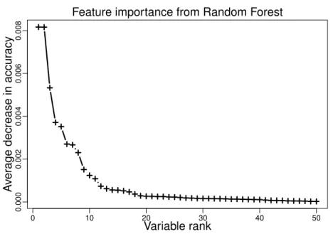
Predictive models built from RF’s top-ranked features usually pro-duce good predictive performances. However, that importance index suf-fers from two main drawbacks that make it bad from an interpretability point of view. Firstly, the ranking of the variables is highly unsta-ble i.e. it may change a lot if the dataset changes a bit. Secondly, it is very difficult to decide which features actually play a role in the decision process. In particular, there is no easy way to define an importance threshold that separates relevant features from irrelevant ones. Indeed, this importance index expresses on a scale which is hardly interpretable.
This thesis provides solutions to these two problems. We perform an analysis of Random Forest stabilities and show how to improve fea-ture selection stability. We propose a statistically interpretable feafea-ture importance index for tree ensemble methods. It outputs p-values that variables are important in the decision process. Altogether, this greatly improves the interpretability of feature selection from tree ensemble methods. In a biomedical context, a stable variable ranking guides the physicians’ investigations. Moreover, they can focus their research on variables that significantly play a role in the medical process.
1.5.2 Kernel methods: new feature selection schemes
The most simple classifiers perform classification by looking for a lin-ear separation between two classes. Support Vector Machines [Vap95] (SVM) is a popular example that is particularly robust to overfitting. It chooses the hyperplane that maximises the margin between the training instances and the decision boundary. SVM can also perform efficient non-linear classification using implicit feature maps through kernels. It simply searches for a linear separation in a projected feature space.
The use of kernels is not restricted to continuous variables. They can be defined for a lot of data types e.g. graphs, pictures, strings, . . . , and of course, categorical data. Combining different kernels enables
classification from heterogeneous data. However, heterogeneous feature selection through kernels remained unexplored.
We ventured on this side and propose two feature selection methods that combine continuous and categorical kernels to handle both kinds of variables. They provide computationally efficient feature selections that reach state-of-the-art performances.
1.6
Summary of the contributions
This section introduces the contributions of this thesis. The main related papers are integrally transcribed in Part III.
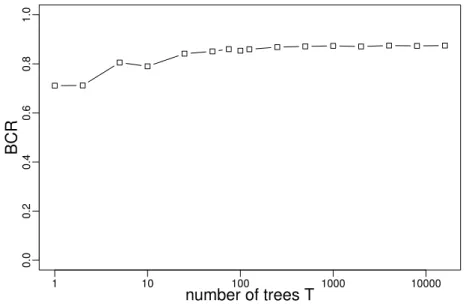
An analysis of tree ensemble methods stabilities Tree ensemble classifiers are known to increase in predictive performances up to a cer-tain point with the number of trees. In [PVD12], we also analyse how the individual sample class predictions and the stability of feature selec-tion improve with the forest size. When dealing with high-dimensional datasets, we show that a very large number of trees are needed to obtain stable feature selection.
Significant features from Random Forest Random Forest already provides variable importance indices but those are not easily interpret-able in a statistical sense. In [PVD13], we present a methodology to assess the statistical relevance of features inside a forest. In particular, we introduceJχ2, a statistically interpretable feature importance index. It outputs p-values that variables are important in a given forest. To do so, it computes a permutation test on out-of-bag instances inside the forest and assesses the level of significance with a Pearson’sχ2 test. In [PD15, PD14b], we compare Jχ2 to two recent alternatives and show that our index has a lower computational complexity by an order of magnitude while keeping similar performances. The paper [PD15], pub-lished in the Neurocomputing journal, can be found in Part III. It is an extended version of the other published papers.
Heterogeneous feature selection with kernels In [PD14a] and [PDD15], we propose two kernel methods to perform heterogeneous fea-ture selection. We use a dedicated kernel, that handles both continu-ous and categorical variables, and plug it into a recursive feature elim-ination (RFE) procedure in order to perform feature selection. One approach internally uses the kernel weights of a multiple kernel learn-ing model to guide the RFE towards important variables. The other
1.7. Publication list 9 method uses weights from a non-linear support vector machine. These new approaches reach state-of-the-art performances. The Neurocom-puting journal paper [PDD15] can be found in the appendices. It is an extended version of [PD14a] which was presented at the ESANN’14 conference.
1.7
Publication list
1. [PVD12] J´erˆome Paul, Michel Verleysen, and Pierre Dupont. The stability of feature selection and class prediction from ensemble
tree classifiers. In ESANN 2012, 20th European Symposium on
Artificial Neural Networks – Computational Intelligence and Ma-chine Learning, pages 263–268, Bruges (Belgium), 2012
2. [PVD13] J´erˆome Paul, Michel Verleysen, and Pierre Dupont. Iden-tification of statistically significant features from random forest. In ECML workshop on Solving Complex Machine Learning Prob-lems with Ensemble Methods, pages 69–80, Prague, Czech Repub-lic, 2013
3. [PD14a] J´erˆome Paul and Pierre Dupont. Kernel methods for
mixed feature selection. In ESANN2014, 22th European
Sympo-sium on Artificial Neural Networks – Computational Intelligence and Machine Learning, pages 301–306, Bruges (Belgium), 2014 4. [PD14b] J´erˆome Paul and Pierre Dupont. Statistically
interpret-able importance indices for random forests. In BENELEARN
2014, 23rd Annual Machine Learning Conference of Belgium and the Netherlands, page 7, Brussels (Belgium), 2014
5. [PD15] J´erˆome Paul and Pierre Dupont. Inferring statistically significant features from random forests. Neurocomputing, 150, Part B:471–480, February 2015
6. [PDD15] J´erˆome Paul, Roberto D’Ambrosio, and Pierre Dupont. Kernel methods for heterogeneous feature selection. Neurocomput-ing, available online 16 April 2015
1.8
Roadmap
This document takes the form of an article thesis. It is divided in three main parts.
Thefirst part, entitled ‘Background and materials’, presents the con-text of this work as well as the necessary tools our approaches are based on. Chapter 2 defines what is classification and presents some exist-ing approaches that perform classification of heterogeneous data. Then, Chapter 3 introduce feature selection as well as state of the art meth-ods in the context of mixed variables. Chapter 4 is the last one of the
first part. It describes the tools and procedures we use to assess the performances of feature selection methods.
The second part summarises the three contributions of this thesis. Its chapters highlight the main results that were published. Each chapter refers to one or several published papers. Chapter 5 gives an overview of an analysis of tree ensemble methods from a stability point of view. Chapter 6 introduces a statistically interpretable feature importance in-dex for Random Forest. The last contribution is reported in Chapter 7. It presents two new heterogeneous feature selection methods based on kernels. A summary of all the contributions is given in Chapter 8 with a few possible extensions to this work as perspectives.
The third part is a collection of the three main papers published during this thesis. The additional papers listed in the publication list (Section 1.7) are shorter and preliminary versions of those longer arti-cles.
Part I
Chapter 2
Classi
fi
cation
In order to perform classification, a predictive model is learned from training data. A model is an internal representation of the prediction problem that allows us to classify previously unseen samples. As the most important objective of classification methods isgeneralisation, a predictive model should mimic the real world as good as possible.
Lack of data, high dimensionality and noise are the three main op-ponents to this generalisation objective. Indeed, a predictive model learned from afinite amount of data can only represent a partial view of the real world problem. In addition, as explained in Section 1.3, high-dimensionality makes model learning even harder. Finally, one cannot consider that the instances available for training are perfectly neat. For instance, measures can be imprecise, some instances may be
misclassi-fied by experts, or some unobserved variables may play a role in the classification task. To summarise,fitting data perfectly leads to overfi t-ting. Proper learning algorithms need additional hypotheses to estimate good predictive models. Those assumptions, such as the form of the de-cision boundary or the way to choose some parameter when learning a classifier, form what is called the inductive bias.
As this work targets heterogeneous data, we will focus on classifiers that can deal with such data. In particular, we detail tree ensemble and kernel methods on which the work of this thesis is based. This chapter is organised as follows. Section 2.1 introduces what is classifi -cation and some notations that will be useful through this document. Section 2.2 details tree ensemble classifiers. It first describes popular decision tree induction methods and then moves to ensemble learning. Afterwards, we turn our attention to kernel methods. Section 2.3 pic-tures Support Vector Machines and the famous kernel trick to perform
non-linear classification and handle different data types. Section 2.4 de-scribes Multiple Kernel Learning which both learns a predictive model and a kernel from the data. Section 2.5 depicts instance-based methods such as the nearest-neighbour classifier and the learning vector quanti-sation method. Section 2.6 explains the naive Bayes classifier that also provides a way to deal with continuous and categorical variables. Fi-nally, Section 2.7 describes an alternative way to deal with both kinds of features, by resorting on a data recoding.
2.1
De
fi
nition and notations
The essence of supervised learning is to infer general rules from examples. The base material is a set of input data and their desired output. The goal is to find a mapping that not only maps the sample data to their output but also generalise well on new unseen data. In classification, the output variable encodes a class membership. A learning algorithm has to find out how to differentiate between samples of different classes. More formally, it has to estimate a decision function f : D → Y that maps the space of input data Dto response labels inY from afinite set of instances {(x1, y1),(x2, y2), . . . ,(xn, yn)} wherexi ∈D andyi ∈Y.
We consider the common case where a dataset is representable as a matrixXn×p wherendenotes the number of samples andp the number of dimensions. The data point xi is a p-dimensional vector consisting
of various measurements. It corresponds to the i-th line of the matrix. When referring to a particular dimension, we use the notation xj. In
the data matrix X, it corresponds to the j-th column. Each dimension can either be continuous (xj ∈ Rn) or categorical. In the second case,
the variable can only take a finite set of values representing the various categories. There is no notion of order between those categories. A categorical variable should rather be seen as a way to partition instances into different groups. Finally, the value of instance i for feature j is written xij.
When dealing with classification problems, the response variable y encodes the class labels. The notationyrefers to the vector that contains the n labels. The class label associated with instance xi is denoted yi.
By nature, the label variable is categorical. However, when there are only two classes, some methods expectyto be numerical and to encode the two class labels as −1 and 1. Those cases are explicitly mentioned in the text.
2.2. Tree ensemble methods 15
2.2
Tree ensemble methods
Decision trees are popular classification methods because of their sim-plicity. They naturally handle continuous and categorical variables, which makes them good candidates for our purpose. However, even if they correctly model their input data, they have limited generalisa-tion capabilities. In addigeneralisa-tion, decision tree inducgeneralisa-tion methods are very sensitive to the training instances: slightly different data leads to very different predictive models. It is a form of overfitting. Ensemble methods such as Random Forest (RF) [Bre01] take advantage of this instability and drastically improve the predictive performances and robustness of the models by growing many decision trees and taking committee deci-sions.
Section 2.2.1 first describes decision trees in a general way. Then it pictures three specific tree induction methods: CART [BFOS84], C4.5 [Sal94] and cTree [HHZ06]. In Section 2.2.2, we give a generic description of tree ensemble methods. We then refine it for three par-ticular cases: Bagging of trees [Bre96], Random Forest [Bre01] and Ex-tremely Randomised Trees [GEW06]. Finally, Section 2.2.3 discuss some limitations of methods based on decision trees.
2.2.1 Decision trees
As we can see on Figure 2.1, a decision tree is a quite simple and easy to interpret predictive model. Each internal node tests one single variable. A branch corresponds to a set or a range of values for a feature. Each leaf is assigned a class label. In order to make predictions, new samples are brought down to the leaves.
Decision trees are particularly appreciated because they are easy to understand. Indeed, each path from the root node to a leaf can be interpreted as a decision rule. Since there is only one variable per node, the decision boundaries of such trees are very simple. Those are piecewise linear and parallel to the axes, as shown in Figure 2.2.
The induction of decision trees is a recursive process. A general pseudo-code is given in Algorithm 2.1. In each node, a splitting cri-terion is chosen from a learning set S. It is a set of pairs (xi, yi) of
training samples and their associated class labels. In the root node, S contains all the training instances. The set F contains variables that are candidate for splitting. For deterministic tree induction methods, F usually contains all the features of the training instances in S. The splitting rule is found by maximising a quality criterion in function get-Split. This criterion is generally a measure of how much the new split
Sick : 10 Healthy : 7 Smokes Sick : 2 Healthy : 4 Gene g Sick : 6 Healthy : 3 Sex Sick : 6 Healthy : 1 Gene g' no sometimes <=42 >42 F M <=23 >23 Sick : 2
Healthy : 0 Sick : 0Healthy : 4 Sick : 0Healthy : 2
Sick : 6 Healthy : 0 Sick : 0 Healthy : 1 Sick : 2 Healthy: 0 often
Figure 2.1: Example of a decision tree with continuous and categorical attributes. In each internal node, the population is shown in the upper rectangle. The lower rectangle shows the variable which is chosen to make the split. Splitting rules are shown on the edges. The final popu-lation is shown in each leaf, along with its attributed class label in bold.
Classification boundary of a decision tree
Figure 2.2: Two dimensional example of a decision boundary of a clas-sification tree for two continuous variables.
2.2. Tree ensemble methods 17 Algorithm 2.1: DecisionTree(S) : build a decision tree
F ← getVariables(S) // set of all variables
split← getSplit(S,F) //variable + splitting rule
if stop(S,split)then
return leaf(S) //create leaf node and assign a class else
foreach partition k according to splitdo Sk← instances of S that belong to partition k
childk← DecisionTree(Sk)
end end
separates well instances of different classes with respect to the current populationS. ThegetSplit function computes the quality of all possible splits of all variables inF and the best splitting rule is kept in thesplit object. The samples of S are then distributed among the child nodes according to this rule. The whole process is repeated until a stopping criterion is met and leaves are created.
There are various kinds of tree induction methods that mainly differ in the way they choose a variable and perform a split in a node (cf. getSplit function in Algorithm 2.1). It is indeed a crucial point since the tree building process is a greedy top-down search. Once a split is decided, this choice is never questioned ever after.
One difficulty when computing the best split is that both continuous and categorical variables need to be assessed. This leads to different strategies to prevent biasing the search towards a variable type or the other. Some training algorithms, such as C4.5 [Sal94], use multi-way splits for categorical variables and binary splits for continuous features. They resort on a specific evaluation criterion that takes into account the nature of the variables. Other methods, such as CART [BFOS84] or cTree [HHZ06], perform binary splits no matter the feature type. Those strategies are described in the remaining of this section.
CART decision trees
The CART [BFOS84] methodology was proposed by Breiman in 1984. It follows the simple idea that splitting a node should increase its purity, or more precisely, decrease its impurity. This concept of node impurity is based on the class labels of the instances inside a node. It is measured
0.0 0.2 0.4 0.6 0.8 1.0 0.0 0.1 0.2 0.3 0.4 0.5
Gini Node Impurity Index for 2 classes
proportion of class 1 samples
Gini
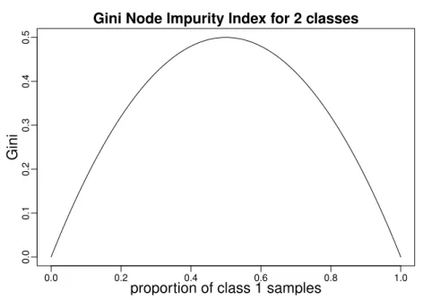
Figure 2.3: Gini index value with respect to the proportion among two classes.
by the following Gini index:
Gini(S) = 1− � c∈classes(S) � |Sc| |S| �2 , (2.1)
where S is the set of learning samples inside a node, Sc is the subset of
samples ofSthat belong to classcand|.|is the set size operator. This index is minimal when the node contains only samples of one class. It reaches a maximum when all classes are equally represented in the setS. As shown in Figure 2.3 for a two class example, the gini index is 0 when the node is totally pure (only one class in the node) and its maximal value is 0.5 when the two classes appear in the same proportions.
The quality of a potential split is given by the difference between the impurity of the parent node and the sum of the impurities of the child nodes. However, if there is no constraints on the number of child nodes, a variable with many different values would artificially lead to a greater drop in node impurity. The more extreme case would be a variable that has a different value for each learning sample, which would lead to |S| child nodes. In that case the drop in Gini would be maximal but this choice most likely overfits the learning data. To overcome this problem, the CART algorithm builds binary decision trees. A graphical example of such tree is given in Figure 2.4. Every node is either a leaf or has
2.2. Tree ensemble methods 19 Sick : 10 Healthy : 7 Smokes Sick : 2 Healthy : 4 Gene g Sick : 8 Healthy : 3 Sex Sick : 8 Healthy : 1 Gene g' no {sometimes,often} <=42 >42 F M <=23 >23 Sick : 2 Healthy : 0 Sick : 0 Healthy : 4 Sick : 0 Healthy : 2 Sick : 8 Healthy : 0 Sick : 0 Healthy : 1
Figure 2.4: Example of a binary decision tree with continuous and cate-gorical attributes. In each internal node, the population is shown in the upper rectangle. The lower rectangle shows the variable which is chosen to make the split. Splitting rules are shown on the edges. The final population is shown in each leaf, along with its attributed class label in bold.
exactly two children, no matter the kind of variable used for splitting. The two children are often referred to as ‘left’ and ‘right’ child nodes. The split quality criterion is therefore defined as follows:
Drop(S, Sl, Sr) = Gini(S)−|
Sl|
|S| Gini(Sl)−
|Sr|
|S| Gini(Sr), (2.2) where S is the set of samples that lie in a given node andSl (resp.Sr)
is the subset of S that goes to the left (resp. right) child-node.
Two different strategies are needed to perform binary splits with continuous and categorical variables. Splits based on a continuous fea-ture are made according to a threshold t. The instances for which the variable of interest has a lower value go in one child node and those with a higher value go to the other. In the case of categorical variables, the set of their possible values is partitioned in two subsets. The instances are thus spread among the two child nodes by comparison to those two sets. Algorithm 2.2 refines the general decision tree description given in Algorithm 2.1 in the case of CART decision trees. It shows how bi-nary splits are made for each variable type. In the pseudo-code, the
function getVariables(S) returns all the variables of the learning sample S i.e. F = {xi | i ∈ [1, p]}. The function getSplit(S,F) measures the
Gini drop (Equation 2.2) of all possible splits of all variables and re-turns the best splitting rule. For each continuous variable in F, it sorts the instances in S and evaluates the|S|−1 thresholds that are midway between two consecutive samples. For the categorical features in F, it computes the Gini drop for each different way to partition the feature values in two sets.1 To reduce overfitting, the CART procedure relies on a pre-pruning strategy. It prevents a node from further splitting when it is sufficiently pure (Gini(S)<α) or when it contains less than a
prede-fined number of samples (|S|< n0), withαand n0 as meta-parameters. Function stop(S,split) halts the growing process whenever one of those criteria is met or if no further split is possible.
Algorithm 2.2: CART(S) : build a CART decision tree F ← getVariables(S)
split← getSplit(S,F) //variable + splitting rule
if stop(S,split)then
return leaf(S) //create leaf node and assign a class else
xj ←split.variable
if xj is categorical then
L←split.leftValues //subset of values ofxjfor left child node
Sxj∈L← subset of S that havexj ∈L
Sxj∈/L←S\Sxj∈L childxj∈L← CART(Sxj∈L) childxj∈/L← CART(Sxj∈/L) else // xj is continuous t←split.threshold
Sxj≤t← instances ofS that have a value≤t forxj
Sxj>t ←S\Sxj≤t
childxj≤t←CART(Sxj≤t)
childxj>t ←CART(Sxj>t)
end end
1For two-class problems, a possible optimisation is to sort the categories according to the probabilities of one class. The optimal split then lies between two positions of the ordered list.
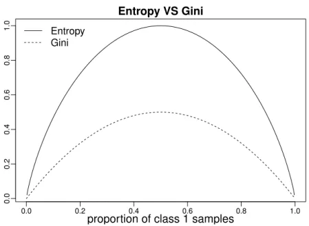
2.2. Tree ensemble methods 21 0.0 0.2 0.4 0.6 0.8 1.0 0.0 0.2 0.4 0.6 0.8 1.0 Entropy VS Gini
proportion of class 1 samples
Entropy Gini
Figure 2.5: Comparison between the entropy and the Gini index with respect to the proportion among two classes.
C4.5
Contrarily to the CART methodology, the C4.5 [Sal94] algorithm does not grow binary trees. It is an extension of the basic ID3 [Qui86] algo-rithm which only considers categorical variables. In that method, one child node is created per possible value of the splitting variable. C4.5 additionally handle continuous variables. This method is described here-after.
Like CART, the idea is to recursively improve the classification of training samples while further splitting nodes. C4.5 uses the entropy as node quality criterion. Its mathematical definition is given hereafter:
Entropy(S) = � c∈classes(S) −|Sc| |S| log |Sc| |S|. (2.3)
This measure captures the quantity of information in knowing the class label of one sample of the setS. For a two-class problem, optimising the entropy is the same as optimising the Gini index (Equation 2.1). Those two measures behave the very same way, as shown in Figure 2.5. The scale is however different. The entropy culminates at 1 while the Gini index has a maximum of 0.5.
The big difference with the CART method is that C4.5 grows multi-way splits for categorical variables. Whenever such split occurs, one child
node is created per category. That way, categorical features appear only once in the decision tree. For continuous features, a binary split is made according to a threshold, similarly to CART. As explained in previous section, this varying number of child nodes calls for an adapted metric in order to assess the split quality: the GainRatio index. It is defined as: Gain(S,{S1, . . . , SK}) = Entropy(S)− K � k=1 |Sk| |S| Entropy(Sk), (2.4) SplitInfo(S,{S1, . . . , SK}) = K � k=1 −|Sk| |S| log |Sk| |S|, (2.5) GainRatio(S,{S1, . . . , SK}) = Gain(S,{S1, . . . , SK}) SplitInfo(S,{S1, . . . , SK}), (2.6)
where Entropy is defined like in Equation 2.3, |.|denotes the set size operator and the sets S1, . . . , SK are the respective populations of the
K child nodes. Those sets form a partition of S. Gain computes the gain in entropy with respect to the class labels when splitting. It is equivalent to the Gini drop (Equation 2.2) in the CART methodology. SplitInfo computes the entropy of the split with respect to thevaluesof the splitting attribute. It can be seen as the quantity of information that one gets in knowing the child node in which one sample of S falls into. Finally, GainRatiois a rescaled gain in entropy that discourages the use of attributes with many values by dividing the gain by the entropy of the split.
The general pseudo-code to grow C4.5 trees is given in Algorithm 2.3. It details how continuous and categorical splits are handled. In compar-ison with Algorithm 2.2, only the categorical split part changes. The C4.5 procedure basically builds full trees. The stop function only halts the tree growing process whenever no additional split is possible. In order to reduce overfitting, a post-pruning strategy based on cross-validation removes nodes in the tree afterwards.
Conditionally independent recursive partitioning
The choice of splitting variables is essential during the tree growing process. It greatly influences the generalisation capabilities of decision trees. However, simple experiments exhibit some biases that depend on the variable type for popular tree learning methods. For instance in [Loh10], the author shows that C4.5 and CART both prefer categorical variables with a high number of possible values. CART also favour continuous features over variables with few categories. Those biases
2.2. Tree ensemble methods 23
Algorithm 2.3: C4.5(S) : build a C4.5 decision tree F ← getVariables(S)
split← getSplit(S,F) //variable + splitting rule
if stop(S,split)then
return leaf(S) //create leaf node and assign a class else
xj ←split.variable
if xj is categorical then
foreachv ∈xj do
Sxj=v ← instances of S that have value v forxj
childxj=v ← C4.5(Sxj=v)
end else
// xj is continuous
t←split.threshold
Sxj≤t← instances ofS that have a value≤t forxj
Sxj>t ←S\Sxj≤t
childxj≤t←C4.5(Sxj≤t)
childxj>t ←C4.5(Sxj>t)
end end
come from the search over all possible splits for each variable. Features with more possible splits have a higher chance to maximise the splitting criterion.
To neutralise this bias, a conditional inference framework for recur-sive partitioning was proposed in [HHZ06]. It relies on a conditional independence test that is performed for each variable in each node of the tree. It tests if variables are independent with respect to the class labels.
Basically, the pseudo-code for growing those trees is similar to CART in Algorithm 2.2. The only differences lie in getSplit and stop where these permutation tests take place both to choose the splitting variable and to halt the process when no feature is significantly dependent of the class labels. From a usability point of view, even if the computational complexity is similar to growing traditional CART trees, the conditional independence tests performed for each variable in each node significantly increase the computational time.
2.2.2 Ensemble of trees
Ensemble methods are based on the idea that asking a committee of experts is better than asking only one. Because of their personal back-ground and experience, experts may have different opinions about the same problem. They would need to argue and discuss to come up with a common solution that takes into account the various views.
The key aspect in such kind of strategy is to mix different points of view on the problem to reach a consensus. With ensemble classifi -cation methods, this is mimicked by building several base learners and promoting diversity among them. In bagging [Bre96] for instance, base classifiers are built from different subsets of the training data. The global decision to classify a new sample is taken democratically from all base learners, by a majority vote. This prevents overfitting and approximates the true class distribution better.
Ensemble methods particularly improve predictive performances over a simple classifier when the base predictors are very sensitive to changes in the dataset. They were even shown to benefit from base classifiers that overfit the learning data [SK96]. That is why several successful en-semble methods are based on unpruned decision trees. This allows us to build more complex decision frontiers while being robust to overfitting (cf. Figure 2.6). However, the main drawback is that predictive models become more complicated. In particular, if a single decision tree is quite easy to interpret in terms of decision rules, it is more difficult to gain insight into an ensemble of trees.
2.2. Tree ensemble methods 25
●
●
●
●
●
●
●
●
●
●
●
●
●
●
●
●
●
●
●
●
●
●
4.5 5.0 5.5 6.0 6.5 2.0 2.5 3.0 3.5 4.0Decision boundaries : RF VS CART
Sepal.Length
Sepal.Width
RF CART
Decision boundaries : RF VS CART RF CART
Figure 2.6: Decision boundaries of a single CART decision tree and a Random Forest. Top: models built on a random two-dimensional subset of Fisher’s Iris [Fis36] dataset. Bottom: 2D artificial dataset where the true class frontier is a circle (classes shown in white and grey).
A generic pseudo-code for growing an ensemble of decision trees from a learning set S ={(xi, yi) |i ∈[1, n]} is given in Algorithm 2.4. The sample function is intentionally left abstract. It could return the full set of instances S or a sub-sample, with or without repeated elements.
Algorithm 2.4:BuildTreeEnsemble(S) : build an ensemble ofT decision trees
fork= 1 to T do
Bk ←sample(S) // bag
Bk ←S\Bk // out-of-bag
hk ←BuildTree(Bk) // see Algorithm 2.1
end
Tree ensemble methods typically grow unpruned decision trees to increase their high variability. In Algorithm 2.1, the training instances are partitioned until no additional split is possible (cf. stop function). In order to grow different base learners, popular tree ensemble methods introduce some randomness in the forest growing process. There are essentially three key points which can be randomised:
1. the bag (set of training instances) of each tree cf. Bk← sample(S) in Algorithm 2.4
2. the set F of candidate variables for splitting in each node cf. F ← getVariables(S) in Algorithm 2.1
3. the way to define the split in each node cf. split← getSplit(S,F) in Algorithm 2.1
Three major approaches, Bagging [Bre96], Random Forest (RF) [Bre01] and Extremely Randomised Trees (Extra-Trees) [GEW06] fall into this framework. Bagging builds multiple trees from randomly selected train-ing instances (point 1). The RF algorithm relies on points 1 and 2 while Extra Trees injects randomness in points 2 and 3.
All those methods grow several trees to form an ensemble classifier that makes predictions based on a majority vote. Even though they could use any kind of decision trees as base learners, they generally grow CART trees. The three methods are described hereafter.
Bagging
The bagging procedure was proposed by Breiman in [Bre96] as a simple way to improve predictive performances over single classifiers. Its name
2.2. Tree ensemble methods 27 is a shortened version of ‘bootstrap aggregating’. While it is originally defined for all kinds of predictor, we focus here on bagging of decision trees.
The bagging method growsT decision trees from different learning sets, or bags. Since they are highly sensitive to the training data, the decision trees are expected to be different and to model different parts of the data. In Algorithm 2.4, each bag Bk is built fromn samples which
are drawn uniformly at random from the dataset S, with replacement. It results in bags containing as much training instances as the original training set. This sampling procedure is known as bootstrap [ET94]. Because samples are taken with replacement, each Bk contains a subset
ofS with some instances appearing multiple times. Indeed, each sample has roughly a 63.2% chance to be part of a specific bag. The instances that are not used to grow the k-th tree form the out-of-bag Bk. They
can be used to obtain internal estimates of the aggregated predictor accuracy.
Random forest
To promote diversity among its decision trees, RF [Bre01] introduces randomness in two different ways. Firstly, following the bagging strat-egy [Bre96], the learning set Bk of each tree is made from a bootstrap
sample [ET94] of the training set S (see Algorithm 2.4). Decision trees are fully grown, following the CART procedure (cf. Algorithm 2.2), without any kind of pruning. Secondly, the splitting criterion is also
randomised. In each node of each tree, a subset F of m ≤ p
candi-date variables is sampled uniformly at random, without replacement. The methodology to find the best split is the same as for the original CART algorithm (see Section 2.2.1) i.e. the drop in node impurity is maximised. However, onlym randomly sampled features are considered instead of the whole set of p variables. This reduces the possibilities to find the best split which further increases the variability in the tree building process. The number m of sampled features is generally quite small with respect to the total number of dimensions p. It is typically set to m=√p.
RF were shown to be very efficient classifiers with very few meta-parameters to tune. In particular, the predictive performances increase
with the number of trees up to a certain point. The number m of
variables to be considered for splitting a node is quite robust. A forest of a few hundreds trees with a default value of√pfor parametermusually performs well for most classification tasks. Those elements make RF a very goodfirst candidate to test if a dataset contains some signal about
class labels.
An ensemble of trees is much more difficult to interpret than a single decision tree. To remedy this situation, the author of the original RF paper [Bre01] proposes a way to estimate the importance of the different variables in the decision process. This is detailed in Chapter 3.
Extremely randomised trees
Like RF, Extra-Trees [GEW06] grows CART-like decision trees. Yet, this algorithm has a slightly different randomisation scheme. It replaces the bootstrap sampling of instances to form each bag by a more random split selection in each node.
With Extra-Trees, each tree is grown from the full learning sample S i.e. Bk = S = {(xi, yi)}ni=1 in Algorithm 2.4. In order to grow dif-ferent decision trees, some randomness is introduced when choosing the decision rule in each node of each tree. First, like in RF,mvariables are chosen at random to form the set F of candidate variables for splitting. Then, for each variable inF, a random cut-point is chosen. Among the m candidate decision rules, the one which maximises the drop in node impurity (Equation 2.2) is kept as the splitting rule of that particular node.
In comparison with RF, the splitting criterion in each node of each tree is thus more randomised. Indeed, RF evaluates all possible splits for each of the candidate features inF while Extra-Trees only considers one possible split per feature. This somehow compensates the fact that, unlike RF, Extra-trees grows all base learners from the same learning sample.
2.2.3 Limitations of approaches based on decision trees
As previously mentioned, the choice of the splitting variable in each node of a tree may be biased with respect to the nature of the candidate fea-tures. This problem is addressed in [HHZ06] where an unbiased scheme is proposed for tree induction at the expense of the computational time. Another limitation comes from the very induction principle of de-cision trees. They may fail to uncover the class signal when it is ‘too multivariate’. Indeed, the recursive partitioning of the data follows a greedy selection mechanism. The first variable at the root node is cho-sen from a strictly univariate criterion. Deeper in the tree, the popula-tion inside a node is condipopula-tioned by the splits above it. However, the splitting variable will still be the one with the biggest univariate effect on that population. It follows that a multivariate class signal (i.e. that one would get by jointly considering several features) might be masked
2.3. Support vector machines 29 because a weaker but univariate signal is preferred by the training algo-rithm.
An illustrative but quite artificial example is given in Figure 2.7. This is a 3 dimensional classification problem with two classes. On the one hand, features x1 and x2 lead to perfect classification when considered jointly. Yet, there is no class information when those features are taken individually. On the other hand, variable x3 convey some class signal but it cannot perfectly predict the two labels on its own. In this case, a tree learning algorithm would selectx3 as splitting variable for the root node, possibly breaking the multivariate signal in x1 and x2.
We observe the same drawback with tree ensemble classifiers. While the random sample selection at the core of bagging methods could induce some marginal effect in features such asx1 andx2, ensemble approaches also miss strong multivariate interactions in the presence of other noisy variables [AN09]. It is particularly true for high dimensional datasets with few samples, such as biomedical data. Some, more complex, alter-natives try to palliate this problem. For instance, one can rely on an exhaustive search of the pairs of possible interacting variables [AN09]. It is also possible to build multivariate splits in each node e.g. with a regression [MKS+11].
2.3
Support vector machines
Support Vector Machine (SVM) [BGV92] is arguably one of the most famous classification algorithms. It is an elegant method that produces state-of-the-art performances, especially with high dimensional biomed-ical data [BHOS+08, Muk03]. In addition, it is quite resistant to
over-fitting and produces very lightweight models. In this section, we give an overview of the SVM classifier from a mathematical point of view. The interested reader is referred to the book of Christopher Bishop [Bis07] for more details. We willfirst describe linear SVM (Section 2.3.1). Then, Section 2.3.2 explains how to perform non-linear classification by pro-jecting the data into a new feature space through the kernel trick. Fi-nally, Section 2.3.3 will present soft-margin SVM that can find a pre-dictive model even if the data is not linearly separable in the feature space.
2.3.1 Linear SVM
In its simplest form, SVM performs binary classification by building a hyperplane that separates two different classes. Such boundary is called a linear discriminant. In two dimensions it is a straight line.
XOR problem
Histogram of for each class
Figure 2.7: Classification problem with 3 variables. The two classes are represented by the different dot and line styles.
2.3. Support vector machines 31 In three dimensions, it is a plane. In p dimensions, it’s a subspace of dimensionality p −1. In this section, we consider that the two class labels are scalars and take values 1 and −1.
Formally, for a binary classification problem, a linear discriminant can be described as a function of a data sample x∈Rp
g(x) =�w,x�+w0, (2.7)
where w is a weight vector in Rp, w
0 a scalar and � , � denotes the scalar product. When g(x) = 0, the sample x lies on the separating hyperplane. The decision rule to classify new samples is
f(x) = sign�g(x)� = � −1 ifg(x)<0 1 ifg(x)>0. (2.8)
In order to reduce overfitting, SVM chooses the maximal margin hyperplane. For a given set of points, the margin is the distance between the hyperplane and its closest points. Those points are the support vectors. They are the only ones that actually matter to express the decision function.
The SVM method is formulated as an optimisation problem. It is detailed hereafter.
Primal
The SVM algorithm looks for the separating hyperplane that has the largest margin under constraints that it separates well instances from different classes. By convention, the support vector lie at a distance g(x) = 1 from the linear decision boundary. The size of the margin is thus �w1�. A graphical example of maximal margin hyperplane is given in Figure 2.8.
In order to maximise the margin, one has to minimise �w�. For mathematical convenience, we minimise 12�w�2 which is an equivalent objective. The SVM optimisation problem is defined as follows:
min w 1 2�w� 2 s.t. yi(�w,xi�+w0)≥1, ∀i∈[1, n], (2.9)
where the constraints simply state that the training samples have to lie in the correct side of the hyperplane, outside of the margin.
Maximal margin hyperplane
Figure 2.8: Two dimensional example of a linear separator that max-imizes the distance betwe

![Figure 2.6: Decision boundaries of a single CART decision tree and a Random Forest. Top: models built on a random two-dimensional subset of Fisher’s Iris [Fis36] dataset](https://thumb-us.123doks.com/thumbv2/123dok_us/474994.2556157/38.892.215.680.253.868/figure-decision-boundaries-decision-random-forest-dimensional-fisher.webp)