Michigan Technological University Michigan Technological University
Digital Commons @ Michigan Tech
Digital Commons @ Michigan Tech
Dissertations, Master's Theses and Master's Reports2018
Resource Optimization in Wireless Sensor Networks for an
Resource Optimization in Wireless Sensor Networks for an
Improved Field Coverage and Cooperative Target Tracking
Improved Field Coverage and Cooperative Target Tracking
Husam SweidanMichigan Technological University, [email protected]
Copyright 2018 Husam Sweidan
Recommended Citation Recommended Citation
Sweidan, Husam, "Resource Optimization in Wireless Sensor Networks for an Improved Field Coverage and Cooperative Target Tracking", Open Access Dissertation, Michigan Technological University, 2018. https://digitalcommons.mtu.edu/etdr/628
RESOURCE OPTIMIZATION IN WIRELESS SENSOR NETWORKS FOR AN IMPROVED FIELD COVERAGE AND COOPERATIVE TARGET TRACKING
By
Husam I. Sweidan
A DISSERTATION
Submitted in partial fulfillment of the requirements for the degree of DOCTOR OF PHILOSOPHY
In Electrical Engineering
MICHIGAN TECHNOLOGICAL UNIVERSITY 2018
This dissertation has been approved in partial fulfillment of the requirements for the Degree of DOCTOR OF PHILOSOPHY in Electrical Engineering.
Department of Electrical and Computer Engineering
Dissertation Advisor: Dr. Timothy C. Havens
Committee Member: Dr. Aurenice M. Oliveira
Committee Member: Dr. Laura E. Brown
Committee Member: Dr. Zhaohui Wang
Dedication
This thesis is for Mom, Dad and Siblings
Contents
List of Figures . . . xiii
List of Tables . . . xix
Preface . . . xxi Acknowledgments . . . xxiii List of Abbreviations . . . xxv Abstract . . . xxvii 1 Introduction . . . 1 1.1 Coverage Optimization in a WSN . . . 2
1.2 Sparse Sensing and Measurement Scheduling . . . 6
1.3 Publications . . . 7
2 Coverage Optimization in a Terrain-Aware Wireless Sensor Net-work . . . 9
2.2 Related Work . . . 11 2.3 Problem Structure . . . 13 2.3.1 ROI Coverage . . . 13 2.3.2 Mobility Cost . . . 15 2.3.2.1 Traveling Distance . . . 15 2.3.2.2 Terrain Severity . . . 16 2.3.3 Objective Function . . . 17 2.4 Algorithms . . . 17
2.4.1 Artificial Immune System Algorithm . . . 18
2.4.1.1 Fitness Proportionate Selection . . . 19
2.4.1.2 Replication . . . 19
2.4.1.3 Clonal Proliferation . . . 20
2.4.1.4 Hypermutation . . . 20
2.4.1.5 Mutation . . . 20
2.4.2 Normalized Genetic Algorithm (NGA) . . . 21
2.4.2.1 Minimum Distance (MINDIST) Normalization . . . 22
2.4.2.2 BLX-α Crossover . . . 23
2.4.2.3 Gaussian Mutation . . . 23
2.5.2 Experiment 2 . . . 28
2.5.3 Experiment 3 . . . 30
2.6 Conclusion . . . 32
3 Sensor Relocation for Improved Target Tracking . . . 35
3.1 Introduction . . . 35
3.2 Problem Statement and Assumptions . . . 40
3.3 Tracking Algorithm . . . 42
3.3.1 Distributed Extended Information Filter . . . 42
3.3.2 Active Set Selection . . . 46
3.4 ROI Formation . . . 49
3.4.1 Kernel Density Estimation . . . 51
3.5 Senors Relocation . . . 52
3.5.1 Sensors Attraction . . . 52
3.5.2 Sensor Position Optimization . . . 53
3.5.3 Fitness Functions . . . 54
3.5.3.1 geometric Dilution of Precision . . . 54
3.5.3.2 Coverage Rate . . . 55
3.5.3.3 Mobility Cost . . . 57
3.5.4 Objective Function . . . 58
3.6 Simulation and Results . . . 58
4 Dynamic Greedy Scheduling for Sparse Sensing in Hybrid Sensor
Networks . . . 67
4.1 Introduction . . . 67
4.2 Problem Setup . . . 73
4.2.1 Simulated Ground-Truth Data . . . 75
4.3 Dynamic Measurement Scheduling . . . 80
4.3.1 Step 1: Measurement Acquisition . . . 80
4.3.2 Step 2: UpdatingΨ(t) and ¯x . . . . 81
4.3.3 Step 3: Reconstruction . . . 82
4.3.4 Step 4: Update Measurement Schedule . . . 84
4.3.4.1 Frame Potential . . . 84
4.3.4.2 Correlation . . . 86
4.4 Results and Discussion . . . 86
4.4.1 Experiment 1 . . . 88 4.4.2 Experiment 2 . . . 90 4.4.3 Experiment 3 . . . 91 4.4.4 Experiment 4 . . . 92 4.4.5 Experiment 5 . . . 93 4.5 Conclusion . . . 94
5.1 Introduction . . . 97
5.2 Formalization . . . 100
5.2.1 Markov Decision Process . . . 101
5.2.2 Inverse Reinforcement Learning . . . 103
5.2.3 Destination Inference . . . 105
5.3 Ground-Truth Data Generation . . . 107
5.4 Feature Generation . . . 109
5.5 Simulations and Results . . . 111
5.6 Conclusion and Future Work . . . 115
6 Conclusion an Future Work . . . 117
References . . . 121
A . . . 135
B . . . 137
C . . . 139
C.1 Tracking (Phase I) . . . 139
C.1.1 Complexity Analysis (DEIF) . . . 140
C.1.2 Complexity Analysis (GNS) . . . 141
C.2 KDE (Phase II) . . . 142
C.4 Execution Time (Phase II and Phase III) . . . 144
List of Figures
2.1 Sensing coverage model. . . 14
2.2 The structure of a population member. . . 18
2.3 Convergence behavior of the optimization algorithms. . . 27
(a) Coverage rate . . . 27
(b) RMS distance . . . 27
(c) Severity . . . 27
2.4 Coverage rate verses the number of sensing nodes N. . . 28
2.5 Impact of the gradient threshold Gth. . . 30
(a) Total severity . . . 30
(b) Total RMS distance . . . 30
(c) Coverage rate . . . 30
2.6 Comparison of the two-point and A-Star scenarios. For the A-star scenario the gradient threshold was Gth = 0.4. . . 31
(a) Severity . . . 31
(b) RMS distance . . . 31
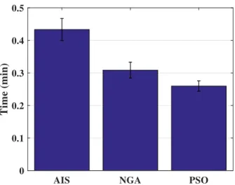
2.7 Comparing the execution time for the three algorithms. Here the
gra-dient threshold was Gth >1, meaning an obstacle free ROI. . . 32
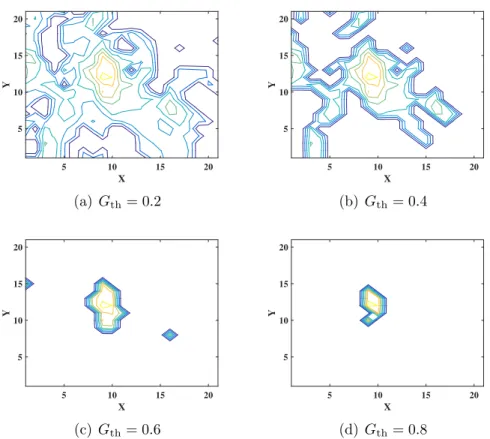
2.8 Obstacles in the ROI for different gradient threshold Gth values. As Gth increases, the number of obstacles in the ROI decreases. . . 33
(a) Gth = 0.2 . . . 33
(b) Gth = 0.4 . . . 33
(c) Gth = 0.6 . . . 33
(d) Gth = 0.8 . . . 33
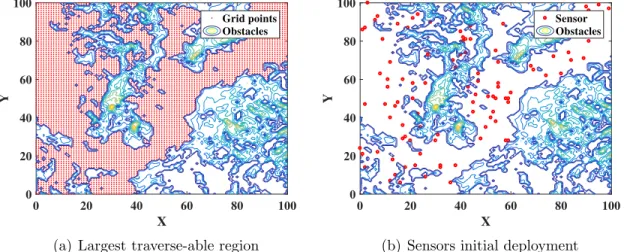
3.1 Initial deployment of sensor nodes in the field’s largest traverse-able region. . . 41
(a) Largest traverse-able region . . . 41
(b) Sensors initial deployment . . . 41
3.2 System flow diagram. . . 41
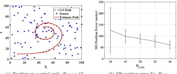
3.3 The impact ofRGNS on the MS position error. . . 49
(a) Tracking on a spiral path. RGNS = 12 . . . 49
(b) MS position error Vs. RGNS . . . 49
3.4 The formation of the ROI based on a fitted model of the estimated targets’ locations. . . 50
(d) ROI centroid . . . 50
3.5 Impact of relocation on missing location estimates. . . 61
(a) Ground-truth tracks . . . 61
(b) Before relocation . . . 61
(c) After relocation . . . 61
3.6 The impact of optimizing the sensors locations inside the ROI as com-pared to only attracting the sensor nodes. Comparison is performed for Rattraction = [0.2,0.25,0.30]. . . 62
(a) RGNS= 5 . . . 62
(b) RGNS= 8 . . . 62
(c) RGNS= 11 . . . 62
3.7 Effect of sensor nodes relocation on field coverage rate. {FROI ← FKcov, RGNS = 8}. . . 63
4.1 Sensing stations in the Melbourne, Australia area / Google Maps. . 71
4.2 Flow diagram of the FFT model for ground-truth data generation. . 76
4.3 Fitting a model for both spatial and temporal variograms. . . 79
(a) Spatial . . . 79
(b) Temporal . . . 79
4.4 Simulated ground-truth data for two time slices. The FFT method was used with the exponential model for both spatial and temporal covariance models. . . 79
(a) . . . 79
(b) . . . 79
4.5 Comparison between the covariance model based on the measured data and the sample-based covariance of the simulated ground-truth data. 80 (a) Spatial covariance . . . 80
(b) Temporal covariance . . . 80
4.6 Flow diagram of the dynamic measurement scheduling. . . 81
4.7 RMSE performance among the various scheduling methods. . . 90
(a) . . . 90
(b) . . . 90
4.8 Comparing the resilience of both the FP and uniform methods to LPS node failure. The x-axis represents the percentage of failed LPS node of the total LPS node count. SNR = 10dB. . . 91
4.9 Impact of HPS nodes percentage (a) and sample size M (b) on the RMSE performance. The FP algorithm is used for scheduling. . . . 92
(a) . . . 92
(b) . . . 92 4.10 Impact of the HPS percentage on the network feasibility. HPS nodes
4.11 Studying the impact of having all the HPS nodes in the active state over the RMSE. M0 indicates an average value. The FP algorithm is
used for scheduling. . . 95
5.1 Impact of the severity control constant η on the generated trajectory. The highereta is, the more sensitive the algorithm is to terrain sever-ity. . . 109
(a) η= 0 . . . 109
(b) η= 0.5 . . . 109
(c) η= 1 . . . 109
(d) Trajectory Statistics . . . 109
5.2 Feature set at states . . . 110
5.3 Trajectory arrangement for result generation. . . 111
5.4 Influence of the trajectory’s observed portion (as a percentage) over the destination prediction accuracy. Methods 1 and 2 are compared. η= 0, β = 0.3. . . 113
5.5 Influence of agent’s sensitivity to terrain on the maximum change in prediction accuracy. β = 0.3. . . 114
(a) Method 1 . . . 114
5.6 The influence the new policy model on the prediction accuracy. Y-axis represents the average accuracy improvement based on ξobserved% =
30% → 90%. Mˆ1 and ˆM2 represent methods 1 and 2 with the new
policy model. β = 0.3. . . 115 (a) . . . 115 (b) . . . 115
List of Tables
2.1 Notations . . . 11
2.2 Parameters Setup for the Two-Point and A-star scenarios. . . 25
2.3 Description of Performed Experiments . . . 26
2.4 Algorithms Comparison. . . 27
2.5 Advantages and Disadvantages of the Presented Algorithms . . . . 34
3.1 Notations Used . . . 39
3.2 Experiments Description . . . 59
3.3 Values of Common Parameters Used in Simulations . . . 60
3.4 Comparing the MS position error (meter) under different optimization methods. RGNS= 8. . . 61
3.5 Impact of RGNS on the coverage rate. The case of initial deployment is considered for illustration purpose. . . 63
3.6 Average cumulative distance (km) traveled by sensor nodes due to relocation (inside ROI) and coverage rate optimization (outside ROI). {FROI ←FKcov, RGNS= 8}. . . 64
4.2 List of covariance models . . . 78
4.3 Experiments Description . . . 88
4.4 Values of Common Parameters . . . 88
5.1 Acronyms and Notations . . . 101
5.2 Experiments Description . . . 112
C.1 Execution Time of a Single Run of the Tracking Algorithm . . . 142
C.2 Computational Complexity of Used Fitness Functions . . . 144
C.3 Execution Time for the Relocation Algorithm Using Different Objec-tive Functions . . . 145
Preface
This work presents an in-depth analysis of some of the most demanding topics in the wireless sensor network (WSN) research domain. Chapter 1 provides an intro-duction to the work presented in the dissertation and lists the main contributions of the different parts seen in the chapters thereafter. The first part mainly addresses the coverage problem for applications related to area-coverage and target tracking. Chapter 2 has been published and presented in the 2016 IEEE Congress on Evolu-tionary Computation (CEC) under the titleCoverage optimization in a terrain-aware wireless sensor network. Moreover, Chapter 3 is published under the titleSensor relo-cation for improved target tracking in the IET Wireless Sensor Systems Journal, April 2018, and the work wasreproduced by permission of the Institution of Engineering & Technology.
The second part of this work investigates the potential gains of introducing a dynamic sparse sensing algorithm into a hybrid WSN framework. The body of the topic is found in Chapter 4, and it was submitted for publication in the IEEE Transactions on Signal Processing on April 2018. Finally, a preliminary work is presented to address the destination prediction problem for mobile targets and the impact a terrain has on the prediction accuracy. This work as seen in Chapter 5 is in preparation to be submitted for publication in a journal addressing related research topics. All the work
in this dissertation was developed under the guidance of my adviser Dr. Timothy C. Havens.
The last chapter provides a conclusion of this work and suggests a set of possible future extensions for the presented material.
Acknowledgments
I would like to start by thanking my advisor Dr. Timothy C. Havens for his guidance, support and mentorship, without which this work would not be possible. It was a true privilege to work with him on several projects, some of which is not presented in this publication. I would also like to thank Dr. Zhaohui Wang for her support and guidance in the early stages of my degree.
The author would like to acknowledge the support of the Electrical and Computer Engineering Department through several research and teaching assistanships.
Finally, many thanks to my family and friends for their encouragement and advice, without which I would not get this far.
The composition of this document and the material presented in Chapter 5 was pos-sible through the Finishing Fellowship awarded by the Graduate School at Michigan Technological University. Superior, a high performance computing infrastructure at Michigan Technological University, was used in obtaining results presented in this publication.
List of Abbreviations
AIS Artificial Immune System BLX Blend Crossover
CS Compressed Sensing
DEIF Distributed Extended Information Filter DKF Distributed Kalman Filter
EM Expectation Maximization FFT Fast Fourier Transform FIFO First In First Out
FIM Fisher Information Matrix FP Frame Potential
GA Genetic Algorithm
GDOP Geometric Dilution of Precision GMM Gaussian Mixture Model
GNS Global Node Selection GPS Global Positioning System GT Ground-Truth
HPS High Precision Sensor IHT Iterative Hard Thresholding
IoT Internet of Things
IPCA Iterative Principle Component Analysis IRL Inverse Reinforcement Learning
KDE Kernel Density Estimation LPS Low Precision Sensor MDP Markov Decision Process MINDIST Minimum Distant
NGA Normalized Genetic Algorithm NP Non-deterministic Polynomial time OLS Ordinary Least Squares
OMP Orthogonal Matching Pursuit PCA Principle Component Analysis PM Particulate Matter
PSD Power Spectral Density PSO Particle Swarm Optimization RMS Root Mean Square
RMSE Root Mean Square Error ROI Region of Interest
SNR Signal to Noise Ratio WSN Wireless Sensor Network
Abstract
There are various challenges that face awireless sensor network (WSN) that mainly originate from the limited resources a sensor node usually has. A sensor node often relies on a battery as a power supply which, due to its limited capacity, tends to shorten the life-time of the node and the network as a whole. Other challenges arise from the limited capabilities of the sensors/actuators a node is equipped with, leading to complication like a poor coverage of the event, or limited mobility in the environment. This dissertation deals with the coverage problem as well as the limited power and capabilities of a sensor node.
In some environments, a controlled deployment of the WSN may not be attainable. In such case, the only viable option would be a random deployment over the re-gion of interest (ROI), leading to a great deal of uncovered areas as well as many cutoff nodes. Three different scenarios are presented, each addressing the coverage problem for a distinct purpose. First, a multi-objective optimization is considered with the purpose of relocating the sensor nodes after the initial random deployment, through maximizing the field coverage while minimizing the cost of mobility. Sim-ulations reveal the improvements in coverage, while maintaining the mobility cost to a minimum. In the second scenario, tracking a mobile target with a high level of accuracy is of interest. The relocation process was based on learning the spatial
mobility trends of the targets. Results show the improvement in tracking accuracy in terms of mean square position error. The last scenario involves the use of inverse reinforcement learning (IRL) to predict the destination of a given target. This lay the ground for future exploration of the relocation problem to achieve improved predic-tion accuracy. Experiments investigated the interacpredic-tion between predicpredic-tion accuracy and terrain severity.
The other WSN limitation is dealt with by introducing the concept of sparse sensing to schedule the measurements of sensor nodes. A hybrid WSN setup of low and high precision nodes is examined. Simulations showed that the greedy algorithm used for scheduling the nodes, realized a network that is more resilient to individual node failure. Moreover, the use of more affordable nodes stroke a better trade-off between deployment feasibility and precision.
Chapter 1
Introduction
The advancements in electronics and communications made it possible to design and build sensory nodes that are compact, power efficient and economically feasible. This paves the road to the utilization of sensory networks in many applications to monitor and record phenomena or a certain activity. To mention few, they can be used for: (1) environmental monitoring of air or water quality, (2) measuring the soil moisture levels in farms, (3) tracking and predicting enemy movement in a war zone. Moreover, the current trends aim at an even more substantial use of sensory networks. The concept of the Internet of Things (IoT) is becoming more predominant in our daily lives. As shown by more and more devices that are equipped to collect and communicate data, like toasters to the vehicles we drive. Sensory networks can be either wired, wireless or a hybrid of both. Wired sensing nodes can be advantageous in terms of having
a more stable power source and communication medium, while wireless nodes offer more flexibility in network’s spatial deployment. This work mainly discusses issues and challenges related to the use of wireless sensor networks (WSN) or the use of wireless nodes to augment a wired sensor network which forms a hybrid network.
Many challenges arise in using a WSN for a given application. Wireless sensor nodes typically have limited resources, namely, battery life, processing power, and sen-sors/actuators capabilities, which leads to: (1) Limited coverage of the event under observation, and (2) a shortened life-time, leading to node failures and hence compro-mising the overall network reliability. This dissertation tackles those challenges by optimizing the use of the available network resources. The sections below present a brief description on how those challenges were addressed, with a more comprehensive discussion provided in the following chapters.
1.1
Coverage Optimization in a WSN
In many scenarios a planned deployment of a WSN can be complicated and unfeasible due to the hostility of the environment. A couple examples of such scenarios would be a sensory network for monitoring an active volcano, or an infiltrator detection and tracking in a war zone. In such cases the only viable option would be an airdrop
distributed network that suffers from coverage holes and connectivity break-offs. Cov-erage holes can lead to a poor depiction of the actual event of interest, and in case of tracking applications an imprecise estimations or utmost a lost tracking. Moreover, having a group of the sensing nodes disconnected due to the random deployment oversight the full potential of the network.
In chapters 2, 3 and 5, the problem of field coverage is addressed from different angles and for different applications. A common theme among those chapters is the study of the impact a terrain has over the proposed methods and solutions. In chapter 2 the problem of sensor relocation after a random initial deployment is tackled. As mentioned earlier, this is of importance due its potential of mending the coverage holes’ problem. The proposed WSN has nodes that are capable of moving across the ROI, but since the the nodes rely on a limited power source, the cost of mobility is high. A multi-objective optimization problem is presented with the purpose of maximizing the area covered by the network, while minimizing the cost of mobility. Mobility cost was introduced to the objective function through both the traveled distance and the severity of the terrain. Due to its relation to the set coverage problem this optimization is considered to be NP-complete, hence the use of evolutionary computation algorithms was considered [14]. Three algorithms were used for this purpose: the Artificial Immune System (AIS) algorithm, the Genetic Algorithm (GA), and the Particle Swarm Optimization (PSO) algorithm . It was shown in the results that both the AIS and GA outperformed the PSO especially
for less dense networks, while the PSO offered a decent performance with a lower execution time [1].
Chapter 3 explores the potential gain of sensor node relocation on the accuracy of target tracking. The nodes in the proposed WSN are assumed to have the ability to be mobile. The presented system is initialized with randomly distributed nodes with the purpose of tracking any moving targets within the field. From this initial state, a database of target location estimates is formed with the intention of using it to learn the mobility trends of the targets of interest. The kernel density estimation (KDE) algorithm is used to estimate a spatial distribution of the previously recorded location estimates, where it is used to establish a ROI the reflects the preferences of the mobile targets. Having established the ROI, the next phase would be relocating a set of sensor nodes to this region, where the nodes are selected based on their distance from the ROI centroid. Several methods are tested to optimize the positioning of the relocated nodes inside the ROI with the intent of achieving a better target position estimates. The first method is based on the geometric dilution of precision (GDOP) metric adapted for our 2D scenario [44]. The GDOP is a dimensionless measure usually used in the satellite navigation domain as an indicate of positioning precision. The second method depends on the K-coverage measure which essentially makes sure that a given point in the field is covered by at least K sensors. Finally, a simple relocation
range [79].
Path and destination prediction for mobile targets has a significant potential in WSNs. For instance, instead of relocating nodes in the whole ROI, it would be more efficient to move a smaller set to cover an area where a target is expected to be. Chapter 5 investigates the use of inverse reinforcement learning (IRL) to predict the destina-tion of a moving target based on observing a pordestina-tion of its trajectory. Targets with different capabilities for traversing a given terrain are considered, where terrain sever-ity is used to generate a set of features with the purpose of learning the preferences and capabilities of the target under investigation. For a varying observed trajectory lengths, the accuracy of prediction is used as a performance measure.
A brief description of the contributions presented in Chapters 2, 3 and 5 are:
† Chapter 2: The use of evolutionary computation to address a multi-objective problem considering a trade-off between coverage rate and mobility cost.
† Chapter 3: Introduce an algorithm for relocating sensor nodes to a region of interest that is deduced based on targets mobility trends, with the purpose of improving the tracking accuracy.
† Chapter 5: Investigating the impact of field’s terrain on the accuray of destina-tion predicdestina-tion.
1.2
Sparse Sensing and Measurement Scheduling
Extending the life-time of a WSN requires a good management of the power resources at the individual node level. It is often common to invest more into optimizing the power consumed by data processing and communications, and less into sensing and data collection. An optimized power management system requires addressing all three areas. In chapter 4 the concept of sparse sensing is introduced to a hybrid network. The hybrid network consists of a sparsely distributed high precision sensor (HPS) nodes, as well as a larger group of low precision sensor (LPS) nodes that are more economically feasible. The goal was to activate a small set of the nodes to measure the phenomena of interest while retaining sufficient information to reconstruct the data of the inactive nodes. Three main methods were investigated to schedule the nodes for measurements: (1) A simple selection of uniformly spaced nodes, and two greedy algorithms with the first based on the (2) frame potential (FP) measure [61, 71], and the other on the (3) correlation measure [72]. The main performance figure of merit was the accuracy of the reconstruction based on the root mean square error (RMSE). Both the uniform and the FP methods offered a superior performance over the correlation approach, with a small edge for the uniform method. Even though the uniform scheduling offered the best reconstruction performance, simulations showed
number of LPS nodes, offered a better balance between reconstruction performance and network deployment feasibility, as compared with an all HPS nodes network. The contribution of as compared to related work in the literature is as follows:
† Introducing the sparse sensing concept into the unique hybrid of LPS and HPS nodes for measurement scheduling, revealing an improvement in reconstruction accuracy while preserving a lower deployment cost.
† Exploring the resilience of the greedy measurement-scheduling algorithms to sensor node failures.
1.3
Publications
The work presented in this dissertation is mainly based on the following publications:
† Chapter: 5
– H.I. Sweidan and T.C. Havens.,”Destination Prediction of Terrain-Aware
Mobile Agents Via Inverse Reinforcement Learning,” In preparation.
† Chapter 4
– H.I. Sweidan and T.C. Havens., ”Dynamic Greedy Scheduling for Sparse
and Remote Sensing.
† Chapter 3
– H.I. Sweidan and T.C. Havens., ”Sensor relocation for improved target
tracking,” IET Wireless Sensor Systems, 2018.
† Chapter 2
– H.I. Sweidan and T. C. Havens.,”Coverage optimization in a terrain-aware
wireless sensor network,” 2016 IEEE Congress on Evolutionary Computa-tion (CEC), Vancouver, BC, pp. 3687-3694. 2016.
Chapter 2
Coverage Optimization in a
Terrain-Aware Wireless Sensor
Network
2.1
Introduction
Regardless of the application for which a wireless sensor network (WSN) is used, coverage is a critical factor that directly impacts the quality of service. There are two main types of WSN coverage addressed in the literature: i) area coverage, where the interest is in maximizing the covered area in a given region of interest (ROI)
[2, 3, 4, 5, 6, 7], and ii) target coverage, where covering static or mobile targets is of essence [8, 9, 10, 11, 12].
For large WSNs, controlled deployment of the sensing nodes not only can be complex, but it is also not practical especially in hostile environments. In such case, random deployment is usually the method of choice. However, random deployment can cause coverage holes, which degrades the effectiveness of the WSN [13]. Therefore, it is necessary to relocate the sensing nodes after the first deployment to mend the coverage holes. In most cases power is a very limited resource in a WSN, where if mismanaged, it would drastically shorten the lifetime of the network. Sensor relocation requires mobility, which is an energy exhausting operation. The amount of energy spent on mobility can be directly associated to: i) traveled distance, and ii) severity of the terrain. Hence, a relocation algorithm is required to maximize the covered area, while keeping the energy spent on mobility at a minimum. This problem is related to the set coverage problems and is considered to be NP-complete [14]. Accordingly, evolutionary computation techniques would be a reasonable choice to investigate this problem.
Table 2.1 provide a description of the important notations used in the following sections. The rest of the chapter is organized as follows. Section 2.2 provides a literature survey for similar problems. The problem structure and the used methods
Table 2.1
Notations
Term Definition Term Definition
Nx,Ny Field dimensions N Number of sensors
Rs Sensing range Rc Communication
range
re Range error P rth Probability threshold a,b Covarience model
pa-rameters
α optimization trade-off parameter
Gth Gradient threshold Ps Population size
Pr Replication rate Pc Clonal percentage
Ph Hypermutation rate Pm Mutation rate
gmax Max. number of
gen-erations
wmin,wmax Inertia limits c1, c2 PSO design
parame-ters
Itrmax Max. number of
iter-ations
work. Simulation results and discussion are found in Section 2.5. Finally, Section 2.6 concludes the work.
2.2
Related Work
Coverage optimization problems for WSNs has been tackled many times in the liter-ature. For limited mobility nodes, an artificial immune system (AIS) algorithm was investigated to maximize the coverage area [2], where the traveled distance was uti-lized as a measure for mobility cost. Yoon and Kim introduced a novel normalization method to thegenetic algorithm (GA), which reduced the redundancy in the solution space resulting in a better performance [3]. Particle swarm optimization has also been examined to resolve the coverage problem. A combination of Voroni diagram
and a two-phase particle swarm optimization (PSO) were used, where the first phase maximizes the coverage area and the second phase minimizes the traveled distance [5]. With regard to target coverage, Zhuofanet al. investigated reducing the mobility cost when solving for both fixed target coverage and network connectivity problems [9]. Mobile target coverage in a vehicular ad hoc sensor network was presented in [11]. This chapter considers the problem of coverage area optimization for sensor relocation after initial deployment. Since energy expenditure of mobility in a WSN is immense, it was penalized by searching for a minimum relocation distance traveled through a terrain with modest severity, where terrain severity is represented by its gradient. Three algorithms are used to inspect this problem, the AIS algorithm, the PSO, and the normalized GA. Although the impact of terrain on sensor deployment has been studied in the literature [15, 16, 17], its impact on the relocation problem requires further investigation. The contribution of the work presented in this chapter reside in the use/comparison of evolutionary computation algorithms to address,
† A multi-objective problem considering a trade-off between coverage rate and mobility cost.
2.3
Problem Structure
2.3.1
ROI Coverage
A square ROI is considered in this work, where aNx×Ny grid is superimposed over
it. Each grid element is of 1×1 size, where a point on the grid is expressed as P(x, y).
N sensing nodes are uniformly distributed in the ROI as an initial deployment, such that sn(xn, yn) is the nth sensor node in the grid, and for simplicity is expressed as
sn. The sensing field of each sensor is considered to be a circle with a radius R.
The probabilistic sensing model is used, where a sensor’s detection uncertainty is accounted for by [2, 18] P rx,y(sn) = 1 R−re ≥d(sn, P), exp−aλb R−re < d(sn, P)< R+re, 0 R+re≤d(sn, P), , (2.1)
where re is the error in the sensing range—see Fig. 2.1. The distance between
sensor sn and point P(x, y) is represented by d(sn, P). The parameters a and b
are for measuring the detection probability in the uncertainty region (i.e., R−re <
Figure 2.1: Sensing coverage model.
probability P rx,y(sn) decays exponentially with distance in the uncertainty region.
The first objective of this problem is to maximize the area covered by the N sensors. It is first required to calculate the coverage rate,
Crate = Carea Atotal
, (2.2)
where Atotal =Nx×Ny is the total area of the ROI. Also, the coverage area Carea is
given by, Carea = Nx X x=0 Ny X y=0 P rx,y(S), ∀P rx,y(S)≥P rth, (2.3)
where S = {s1, s2, ..., sN} is the set of all sensors, and P rx,y(S) = 1− QN
n=1(1− P rx,y(sn)) is the coverage probability of pointP(x, y) considering the sensors inS. If
2.3.2
Mobility Cost
2.3.2.1 Traveling Distance
This work examines two traveling methods. The first is along a two-point path where the first point is the one of initial deployment and the second is the destination. The other method is carried along a path computed using the A-star algorithm to avoid severe terrains—details in Section 2.3.2.2. Obviously the A-star path is at least as long as the two-point path. The traveling distance of relocating the sensors in S is assessed by the root-mean-square (RMS) of their individual traveling distances,
dRMS = v u u t 1 N N X n=1 d(sn, Pn,f)2, (2.4)
wherePn,f is the final point of thenth sensor relocation path. The distanced(sn, Pn,f)
is expressed as, d(sn, Pn,f) = Mn X m=2 p (xm−xm−1)2+ (ym−ym−1)2, (2.5)
where Mn is the number of points on the nth sensor relocation path, with Mn = 2
2.3.2.2 Terrain Severity
Here, the severity of the terrain is mainly quantified by its steepness. For instance, a steep downhill or uphill terrain is considered more difficult to traverse, and hence not preferable for sensors to pass through. Steepness is computed by evaluating the gradient of the terrain and then taking its absolute value. Therefore, the severity of the nth sensor relocation path is given by
Sev(sn, Pn,f) =
PMn
m=1|G(Pn,m)|
Mn
, ∀Mn ≥2, (2.6)
where Pn,m is the mth point on the nth sensor relocation path, and G(Pn,m) is the
gradient at that point. The overall relocation severity can be measured as
SevRMS = v u u t 1 N N X n=1 Sev(sn, Pn,f) 2 , (2.7)
where SevRMS is the RMS of the relocation severity for the sensors in S. When
considering the A-star method, parts of the terrain may be perceived as an obstacle based on the value of gradient. A point P(x, y) in the grid is considered to be an obstacle if
where G0(P(x, y)) is the normalized gradient at point P(x, y), and Gth ∈ [0,1] is a
threshold parameter for the gradient.
2.3.3
Objective Function
For the problem at hand, maximizing the coverage while keeping the mobility cost at a minimum is of interest. Accordingly, the objective function can be expressed as,
min F =αC¯rate+ (1−α) dRMS SevRMS Rc , (2.9)
where α ∈ [0,1] is a design parameter that allows the user to select the trade-off between the coverage and mobility costs. The parameter Rc is the sensor’s
com-munication range, and it is used in the objective function to count for the network connectivity.
2.4
Algorithms
The algorithms used to assess the problem at hand are either evolutionary (GA and AIS) or related to the evolutionary techniques (PSO), where they rely on a population of solutions in the search for optimality. The structure of a member in a population is illustrated in Fig. 2.2.
Figure 2.2: The structure of a population member.
2.4.1
Artificial Immune System Algorithm
The following provides some details regarding the AIS algorithm, outlined in Algo-rithm 1 [2, 19].
Algorithm 1 AIS Algorithm
P oP ← Initialize the population.
2: ng = 0 (generation counter).
while ng ≤gmax do
4: F(S, P oP)←Antibody fitness evaluation.
P oPsel ←Fitness proportionate selection.
6: P oPrep← Replicate best Pr×Ps antibodies.
P oPclo← Apply clonal proliferation over P oPrep.
8: P oPhyp ← Hypermutation overP oPclo. P oPtot ←[P oPrep;P oPhyp].
10: P oPchild ← Mutation over P oPtot.
P oP ← Select BestPs antibodies out of P oPchild.
12: ng =ng+ 1
end while
14: Sfinal← Antibody with the minimum fitness.
2.4.1.1 Fitness Proportionate Selection
The selection process is carried out by first normalizing the fitness value of each antibody in the population,
Fnorm =
F(S, P oP)
PPs
l=1F(S, P oP(l))
, (2.10)
where Fnorm ∈ [0,1] is a vector containing the normalized fitness values, and F(S, P oP) computes the fitness of each antibody in the population. P oP(l) is the
lth antibody in the population, and Ps is the population size. The next step is to
calculate the cumulative sum of the values inFnorm, and then select the first antibody
with a cumulative fitness that exceeds a random number r ∼ U[0,1]. The selection based on the random number r is repeated Ps times and the resulting antibodies are
stored in P oPsel.
2.4.1.2 Replication
ThePsantibodies chosen by the fitness proportionate selection are sorted in ascending
order according to their fitness values, and the first Pr×Ps antibodies are kept in
2.4.1.3 Clonal Proliferation
A random number r ∼ U[0,1] is assigned to each antibody in P oPrep. For the case
where the clonal percentagePc is greater than r, that antibody is placed in P oPclo.
2.4.1.4 Hypermutation
Every antibody that joined the clonal proliferation goes under the hypermutaion process. For an antibody A = {J1J2...Jk...J2N}, any given gene could be chosen
for hypermutation depending on the rate Ph. Assume that gene Jk was chosen for
hypermutation, another geneJi is then randomly selected to join the operation. The
new gene Jk0 = (1−Γ)Jk+ ΓJi, for Γ∼U[0,1], and is stored inP oPhyp.
2.4.1.5 Mutation
Similar to the hypermutation process, mutation promotes exploration through diver-sifying the antibodies. With a ratePm much lower than Ph, mutation is applied over
the antibodies in P oPrep and P oPhyp. For an antibodyA ={J1J2...Jk...J2N}, let Jk
selected from A to join the process. The new mutated genes are expressed as
Jk0 = (1−Γ)Jk+ ΓJi, (2.11)
Ji0 = (1−Γ)Ji+ ΓJk, (2.12)
where Γ∼U[0,1].
2.4.2
Normalized Genetic Algorithm (NGA)
In this type of problem, redundancy imposes itself in the solution (phenotype) space. For instance, let us express a solution (chromosome) Ai in the phenotype space as
a set of 2D location pairs for the sensors in S; Ai = {(x1, y1)(x2, y2)...(xN, yN)}.
Another solution Aj might exist with a set of pairs that are only a rearrangement of
the ones inAi. This will cause similar results in terms of coverage, but not necessarily
in traveling distance or path severity. The normalized GA introduced by Yoon and Kim, outlined in Algorithm 2, addresses this issue [3]. The following provides some details regarding the normalization, crossover, and mutation operations used in this algorithm.
Algorithm 2 Normalized Genetic Algorithm (NGA)
P oP ← Initialize the population.
2: ng = 0 (generation counter).
while ng ≤gmax do
4: {Parents1,Parents2} ← Random pairing.
Parents02 ← MINDIST normalization on Parents2.
6: OffSpring← BLX-0.5 crossover.
OffSpring0 ← Gaussian mutation over OffSpring.
8: P oPtot ←[P oP; OffSpring0]
F(P oPtot,S)← Chromosome fitness evaluation.
10: P oP ← Select bestPs chromosome out of P oPtot. ng =ng+ 1
12: end while
Sfinal← Chromosome with the minimum fitness.
14: return Sfinal
2.4.2.1 Minimum Distance (MINDIST) Normalization
Before starting the MINDIST normalization, it is necessary to randomly pair the Ps
chromosomes into Ps/2 parent pairs. For illustration, let the chromosomes be
repre-sented as a set of 2D location pairs, with Al,1 ={(x1,1, y1,1)(x1,2, y1,2). . .(x1,N, y1,N)}
and Al,2 = {(x2,1, y2,1)(x2,2, y2,2), . . .(x2,N, y2,N)} be the first and second parents in
the lth pair. The MINDIST normalization is carried out by rearranging the pairs in the second parent such that the sum distance between Al,1 and Al,2 is at minimum.
The Euclidean sum distance has the following expression,
N
X
n=1 q
2.4.2.2 BLX-α Crossover
For the parent pair A1 = {J1J2...J2N} and A2 = {L1L2...L2N}, the blend crossover
(BLX) produces the offspring A0 = {M
1M2...M2N} by uniformly selecting the gene
Mn from the range [min(Jn, Ln)−αI,max(Jn, Ln) +αI], where I =|Jn−Ln| and α
is a design variable [3, 20]. A common value for α is 0.5.
2.4.2.3 Gaussian Mutation
The Gaussian mutation is performed on a gene Ji with a mutation rate Pm by
Ji0 = min(max(β, Ji,min), Ji,max), (2.14)
where Ji,max and Ji,min are the upper and lower bound on the gene Ji. Also, β ∼
N(µ, σ) is a normally distributed random number with meanµand standard deviation
σ. In this workµ= 0 andσ = (Ji,max−Ji,min)/10.
2.4.3
Particle Swarm Optimization
Here we consider a simple form of PSO based on the work initially presented by Kennedy and Eberhart [21]. Each sensor in S represents a particle in the swarm.
Updating the velocity and position vectors for the nth particle is carried out as
Vni+1 =wVni+r1c1(Pnbest−P i
n) +r2c2(PG−Pni), (2.15)
Pni+1 =Pni +Vni+1, (2.16)
wherei∈[0, imax] is the iteration counter and wis the inertia; its value changes with
each iteration as w = wmax −(wmax−wmin)imaxi . The values of wmin and wmax are
set to 0.4 and 0.9, respectively [22]. Pbest
n is the point with the best fitness for the
nth sensor, and PG is the point with the best fitness among all sensors (particles).
Velocity limits of Vmin = −0.5(Pmax−Pmin) and Vmax = 0.5(Pmax−Pmin) were used
to initiate particles’ velocities, wherePmin and Pmax are the ROI limits.
2.5
Simulation and Results
For our simulations, two different sets of parameters are used for the problem setup and the used algorithms—see Table 2.2. The first set is for generating results to compare the algorithms in the two-point path case, where no part of the terrain is conceived as an obstacle. The second set of parameters is mainly for investigating the A-star path case, where the presence of obstacles is possible. All terrains used throughout the simulations are synthetically generated. Several PCs were used to
Table 2.2
Parameters Setup for the Two-Point and A-star scenarios.
Two-Point A-Star Problem setup Nx×Ny 51×51 21×21 N 10→70 10 Rs 5 3 Rc 10 6 re 0.6Rs 0.6Rs P rth 0.85 0.85 a 0.5 0.5 b 0.5 0.5 α 0.9 0.9 Gth – [0.2,0.4,0.6,0.8, >1] AIS Ps 50 15 Pr 0.9 0.9 Pc 0.1 0.1 Ph 0.7 0.5 Pm 0.01 0.05 gmax 100 30 PSO Ps 50 15 wmin 0.4 0.4 wmax 0.9 0.9 c1 4 4 c2 2 2 Itrmax 100 30 Ps 50 15 NGA Pm 0.001 0.001 gmax 100 30 GHZ, i7-4770S 3.1 GHZ).
In the following we perform three sets of experiments to compare the presented algo-rithms. Table 2.3 outlines the scenarios for each of the experiments.
Table 2.3
Description of Performed Experiments
Description Parameters Experiment 1 Obstacle-free ROI, where
sen-sors follow a two-point path.
Table 1 (Two-Point) Experiment 2 The ROI can contain obstacles,
and sensors follow a path gen-erated by the A-Star algorithm.
Table 1 (A-Star)
Experiment 3 Comparing the scenarios in ex-periments 1 and 2.
Table 1 (A-Star)
2.5.1
Experiment 1
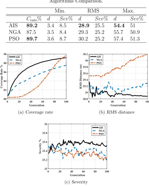
In this experiment a comparison is held among the presented algorithms for the case where no part of the terrain is perceived as an obstacle; hence, sensors are able to follow a two-point path. The parameters used from Table 2.2 are the ones of the two-point case. The results shown in Table 2.4 are generated by averaging 50 runs of each algorithm, with N = 70. It can be seen from Table 2.4 that the AIS algorithm outperforms the other two in terms of traveled distance. Both the AIS and PSO algorithms seem to have better performance in terms of coverage rate than that of the NGA algorithm. With regards to the convergence rate, Fig. 2.3 reveals that for path severity the three algorithms are close to each other and decay at almost the same rate. The AIS algorithm has an obviously better performance in terms of the RMS distance, but slightly falls behind the PSO for the coverage rate especially after
Table 2.4
Algorithms Comparison.
Min. RMS Max.
Crate% d Sev% d Sev% d Sev%
AIS 89.2 3.4 8.5 28.9 25.5 54.4 51 NGA 87.5 3.5 8.4 29.3 25.2 55.7 50.9 PSO 89.7 3.6 8.7 30.2 25.2 57.4 51.3 Generation 0 20 40 60 80 100 Coverage Rate % 80 82 84 86 88 90 AIS NGA PSO
(a) Coverage rate
Generation 0 20 40 60 80 100 RMS Distance (m) 28.8 29 29.2 29.4 29.6 29.8 30 30.2 AIS NGA PSO (b) RMS distance Generation 0 20 40 60 80 100 Severity % 25 25.2 25.4 25.6 25.8 26 AIS NGA PSO (c) Severity
Figure 2.3: Convergence behavior of the optimization algorithms.
can be seen clearly from the divergence of the PSO for the rms distance, and the slow convergence of all three algorithms especially for path severity.
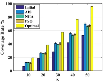
Figure 2.4 examines the impact of increasing the number of sensing nodes N on the coverage rate. The initial coverage rate is that of the first random deployment, and the optimal coverage rate is the one achieved by placing the sensing nodes with an
N 10 20 30 40 50 Coverage Rate % 0 20 40 60 80 100 Initial AIS NGA PSO Optimal
Figure 2.4: Coverage rate verses the number of sensing nodesN.
equal threshold distance dth from each other within an obstacle-free ROI of a regular
shape [2]. Furthermore, in the optimal case the nodes need to have similar sensing radiusRs, and dth=
√
3Rs. All algorithms seem to achieve better coverage rate asN
increases. Even though the PSO algorithm does not perform as well for N < 30, it soon recovers for higher number of sensing nodes. It is clear that the AIS algorithms achieves better coverage than the NGA and PSO algorithms, particularly forN >10. From the previous, the AIS algorithms seems to offer the best compromise; good coverage rate, low rms traveling distance and a comparable path severity.
2.5.2
Experiment 2
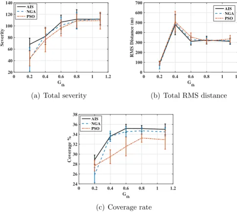
around obstacles. At any generation/iteration, if the solution produces a destination point that is surrounded by obstacles, over an obstacle or on the initial location, no relocation occurs. The parameters used to generate the results for this experiment are found under the “A-star” column in Table 2.2. Figure 2.5 illustrates the impact of varying Gth on the total severity, total RMS distance, and coverage rate. The
total severity is evaluated by summing SevRMS over all generations and the total
distance is evaluated likewise. As observed in Fig.2.5, the three algorithms acquire similar performances in terms of severity and RMS distance. Both the AIS and NGA algorithms outperform the PSO algorithm in terms of coverage rate, especially for
Gth > 0.2, Fig.2.5(c). The closeness in performance between the AIS and NGA
can be referred to the somewhat similar evolutionary framework, as opposed to the swarm evolutionary approach the PSO algorithm is based upon. Moreover, even though the error bars of the PSO coverage curve seem substantial, performing a z-test confirms that it belongs to different distribution . AsGth increases the number of
obstacles decrease, which in effect gives more freedom for the nodes to move around, generating a longer relocation paths. A longer path means larger RMS distance and higher probability of traversing more severe terrains. It is observed from Fig.2.5(b) that the RMS distance peak atGth = 0.4, this is due to obstacles that force the nodes
0 0.2 0.4 0.6 0.8 1 1.2 G th 20 40 60 80 100 120 140 Severity AIS NGA PSO
(a) Total severity
0 0.2 0.4 0.6 0.8 1 1.2 G th 0 100 200 300 400 500 600 700 RMS Distance (m) AIS NGA PSO (b) Total RMS distance 0 0.2 0.4 0.6 0.8 1 1.2 G th 24 26 28 30 32 34 36 38 Coverage % AIS NGA PSO (c) Coverage rate
Figure 2.5: Impact of the gradient threshold Gth.
2.5.3
Experiment 3
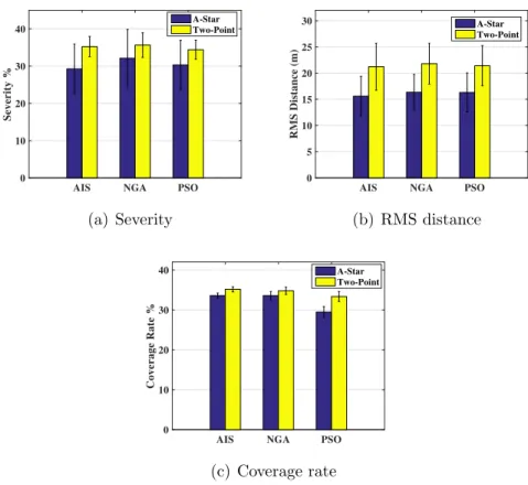
For this experiment, a comparison is made between the two scenarios presented in the first two experiments, but with the parameters of the second experiment applied to both. In Fig. 2.6 a comparison between the utilized algorithms is held for total severity, total RMS distance, and coverage rate withGth = 0.4 for the A-star scenario.
Due to the presence of obstacles in the A-Star scenario, the movement of nodes is limited and hence shorter relocation paths are generated, Fig.2.6(b). A shorter path
AIS NGA PSO 0 10 20 30 40 Severity % A-Star Two-Point (a) Severity
AIS NGA PSO
0 5 10 15 20 25 30 RMS Distance (m) A-Star Two-Point (b) RMS distance
AIS NGA PSO
0 10 20 30 40 Coverage Rate % A-Star Two-Point (c) Coverage rate
Figure 2.6: Comparison of the two-point and A-Star scenarios. For the A-star scenario the gradient threshold wasGth= 0.4.
lower path severity and RMS distance for the A-Star scenario comes at the expense of reduced coverage rate, Fig. 2.6(c). For both scenarios the AIS algorithm seems to outperform the other two in every aspect under consideration.
The execution time of the three algorithms is compared forGth >1 reflecting the case
of an obstacle free ROI, Fig. 2.7. .From the figure, the AIS algorithm possesses the highest execution time while the PSO has the lowest. Taking the two-point scenario into consideration and with same parameters as in experiment 2, all three algorithms execute in a time under 0.9 seconds—for Gth > 1—which is around 95% less. For
AIS NGA PSO Time (min) 0 0.1 0.2 0.3 0.4 0.5
Figure 2.7: Comparing the execution time for the three algorithms. Here the gradient threshold was Gth>1, meaning an obstacle free ROI.
no obstacles present in the ROI, and in the case where the execution time is not of essence, the AIS algorithm would be more preferable, for it has a good coverage rate with reasonable RMS distance and severity, especially in the two-point case.
2.6
Conclusion
For a WSN where the sensor nodes are initially deployed randomly in a ROI of a regular shape, this work addressed the problem of sensor relocation to maximizing the sensing coverage, while maintaining a minimal mobility cost. The cost of mobility was directly associated to the traveling distance and the severity of the relocation path. The terrain severity was characterized based on its gradient. Two main scenarios
X 5 10 15 20 Y 5 10 15 20 (a) Gth= 0.2 X 5 10 15 20 Y 5 10 15 20 (b)Gth= 0.4 X 5 10 15 20 Y 5 10 15 20 (c) Gth = 0.6 X 5 10 15 20 Y 5 10 15 20 (d)Gth= 0.8
Figure 2.8: Obstacles in the ROI for different gradient thresholdGthvalues.
AsGth increases, the number of obstacles in the ROI decreases.
any terrain along their path, and the second considered the case where nodes might not be able to pass through certain terrains, which gives rise to obstacles. In the first scenario the relocation path was considered as a straight line defined by two points, and in the second the A-star algorithm was used to generate a path capable of maneuvering obstacles. Results show that there is no single algorithm that surpasses the others in all cases and scenarios. Having said that, the AIS algorithm seems to offer the best compromise between coverage rate and cost of mobility. Even though the AIS algorithm has the longest execution time, for the relocation problem this might not be a crucial factor. Table 2.5 provides the advantages and disadvantages
Table 2.5
Advantages and Disadvantages of the Presented Algorithms
Advantages Disadvantages AIS Best coverage rate for most values of
N.
Low traveling distance.
Slightly higher path severity than NGA and PSO.
High execution time. NGA Good coverage rate especially for
lowN.
High execution time, but lower than AIS.
PSO Low execution time. In general has lower coverage rate. of the presented algorithms in the context of our problem.
Chapter 3
Sensor Relocation for Improved
Target Tracking
3.1
Introduction
Due to its importance and influence on the dependability of a wireless sensor net-work (WSN), the coverage problem has attracted much attention in the literature. Depending on the application, sensor deployment can be oriented toward improving
area coverage [2, 23, 24, 25, 26, 27], ortarget/event coverage [18, 28, 29, 30]. In harsh or hostile environments a controlled deployment can be arduous and in some scenarios
not possible. In such a case, the only alternative would be a WSN with randomly dis-tributed sensing nodes, resulting in coverage holes and connectivity problems among the nodes [31]. Hence, a relocation of the sensing nodes might be necessary after the initial deployment to improve the performance of the network. In this note, target tracking is of interest and the quality of tracking is a main objective. Targets usually tend to follow patterns while traveling in a given region; animals travel in routes for food, mating or shelter; troops and artillery in a war zone travel in secure but traverse-able paths. Therefore, it is of interest to learn target trends and relocate the appropriate sensor nodes accordingly. Furthermore, it might be desirable to enhance the tracking quality in a given region of interest (ROI) due to the region’s strategic importance. However, sensor relocation to cover a certain ROI creates coverage holes in other parts of the field, preventing the detection of possible future targets. Hence, it is also important to keep the field coverage rate into consideration. The mobility of sensors is usually expensive in terms of power consumption, therefore it is desirable to keep this cost to a minimum while relocating the nodes. The problem at hand can be related to set-coverage problems which are considered NP-complete [14]. As a result, the use of an evolutionary computation algorithm would be reasonable. For this work, the genetic algorithm (GA) is considered.
at-nodes around the event location with a sensor density that depends on the event intensity. The coverage and monitoring of a large population of objects—mass ob-jects—was investigated from a probabilistic perspective [30]. The authors introduced an online distributed recursiveexpectation maximization (EM) algorithm for dynamic deployment of sensors with the purpose of improving the detection and boundary es-timation of mass objects.
Olfati introduced the flocking concept to the distributed tracking of a target [32]. Even though the flocking behaviour of the mobile sensor network was a byproduct of minimizing the estimation error for each of the nodes, it resulted in a connected network with topologies that improved the performance of the distributed Kalman filter (DKF).
Learning contextual information from an image sequence for improving object-tracking has also been addressed [33, 34]. Gaussian mixture models (GMMs) were used to learn the distributions of the object-birth and clutter events [34]. The learned models were used to adapt the object-tracking filter for an improved performance.
In this work, for a WSN with an initial deployment following a uniform distribution, a distributed extended information filter (DEIF) is used to perform target tracking. The EIF is a variant of the Kalman filter that has been used in the literature in its distributed form for target tracking [35, 36, 37]. Also, the global node selection
localization at the next dynamic step [35]. For the problem at hand, the geometric dilution of precision (GDOP) is used as a basis in the sensor selection algorithm and as an one of the objective functions considered for the sensor relocation process. The GDOP is a dimensionless measure originally used inglobal positioning system (GPS) to select satellites with geometrical positions that offer a more accurate localization [38]. Most related work in the literature only considers optimizing the deployment of the WSN for achieving a better tracking [39, 40, 41]. This has the problem of not being able to adapt to the changes in targets’ characteristics and mobility trends. This work addresses this issue by introducing a relocation algorithm that moves the sensor nodes to a ROI that corresponds to the mobility patterns of the target. Moreover, the impact of the terrain was reflected on the generated ROI. In general, the contribution of this work is summarized by,
† Presenting a relocation algorithm for improving the target tracking accuracy.
† Relocating the sensor nodes to a region of interest that was deduced based on targets mobility trends.
† The presented algorithm is dynamic in the sense that it is capable of relocating the nodes as the targets’ mobility trends changes.
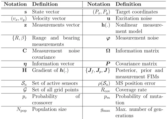
Table 3.1
Notations Used
Notation Definition Notation Definition
s State vector (Px, Py) Target coordinates
(vx, vy) Velocity vector u Excitation noise
z Measurements vector h(.) Nonlinear measure-ment model
{R, β} Range and bearing measurements
ϕ Measurement noise
C Measurement noise covariance
Ω Information matrix
η Information vector P Covariance matrix
H Gradient of h(.) {Jf,Jp,J} Posterior, prior and
measurement FIMs
Sa Set of active sensors ρ(Sa) MS position error
G Set of all grid points Rcov Coverage rate pc Probability of
crossover
pm Probability of
muta-tion
Npop Population size gmax Max. number of
gen-erations
Table 3.1 lists the main notations used throughout this work. The remainder of this chapter is organized as follows. Section 3.2 describes the problem structure as well as the adopted assumptions. The tracking algorithm is presented in Section 3.3. Section 3.4 discusses the formation of the ROI using the kernel density estimator
(KDE) method. The process of sensor relocation and the objective functions used for location optimization are presented in Section 3.5. Section 3.6 describes the experiments performed and offers a discussion for the presented results. Finally, the work is concluded in Section 3.7.
3.2
Problem Statement and Assumptions
In an Nx ×Ny field, a WSN of N sensors (nodes) is deployed where the locations
of the nodes first follow a uniform distribution. Sensors are assumed to be mainly distributed in the largest traverse-able region in the field, avoiding obstacles and locked regions, e.g., see Fig. 3.1. This is a fairly realistic assumption for large fields, as sensors tend to be deployed in regions that are predominantly traverse-able by targets as well as mobile sensor platforms. The setS includes all sensors in the WSN. Sensors are assumed to be time synchronised and each sensor knows the location of all other nodes. The connectivity among the nodes is assumed to be maintained through a multi-hop routing model [42], the details of which are beyond the scope of this chapter. For the purpose of investigating the problem of node relocation, a simple model of a single target with a nearly constant velocity is adopted. Moreover, the measurement model assumes a stationary target. A probabilistic detection model is used, with a probability of one within a predetermined range from the sensor, that afterwards drops exponentially until it reaches zero. The flow diagram for the problem structure is illustrated in Fig. 3.2. Initially, the randomly distributed WSN performs tracking over a given period of time that depends on the activity and nature of targets moving in the field. The purpose of this phase is to collect a database of
is used to specify a ROI of high probability target locations; more details are found in Section 3.4. Finally, the relocation algorithm moves the sensor nodes in a manner that would improve the tracking performance in the constructed ROI; see Section 3.5. Appendix A provides the derivation of the mean square position error, while Appendix B presents a brief discussion of the error propagation throughout the proposed system. The time complexity analysis can be found in Appendix C.
0 20 40 60 80 100 X 0 20 40 60 80 100 Y Grid points Obstacles
(a) Largest traverse-able region
0 20 40 60 80 100 X 0 20 40 60 80 100 Y Sensor Obstacles
(b) Sensors initial deployment
Figure 3.1: Initial deployment of sensor nodes in the field’s largest traverse-able region.
3.3
Tracking Algorithm
For collective tracking of a given target, two main procedures are essential for the tracking algorithm. The first selects a set of sensor nodes used for estimating the target state, while the other carries out the estimation. Next is a brief description of the DEIF algorithm used for target state estimation, and the GNS algorithm used for sensor node selection.
3.3.1
Distributed Extended Information Filter
In this section, a set of equations used for the estimation of a target location using a set of active senors Sa is presented. The target non-linear dynamic system model,
composed of a state equation and measurement equation, is now described. Thestate equation is
sk=Gsk−1+Buk, (3.1)
where the state vector sis
s= Px Py v ,
(Px, Py) are the target coordinates and (vx, vy) are the velocity vector components.
Also,u∼N(0, σ2
uI) is a representation of the target acceleration. Matrices Gand B
are G= 1 0 ∆ 0 0 1 0 ∆ 0 0 1 0 0 0 0 1 , B= 0.5∆2 0 0 0.5∆2 ∆ 0 0 ∆ ,
where ∆ is the step size between two time snapshots. The measurement equation is
z(kj) =h(j)(sk) +ϕk, (3.2)
where the (j) superscript indicates the jth sensor in the setSa.The functionh(.) is
h(s) = p (Px−x)2 + (Py −y)2 arctanPy−y Px−x = R β ,
which represents the nonlinear measurement model, such thatR and β are the range and bearing from a sensor at (x, y) to the target at an estimated position of (Px, Py),
respectively. Also, ϕk ∼N(0,C) is the measurements noise, where
C= σ2 R 0 0 σβ2 .
Here, σR2 and σβ2 are fixed among the sensors at all times. Even though the measure-ment model h(.) does not take into consideration the target mobility, the simulated
bearing measurements did incorporate the target non-stationarity, see equation (3) in [35]. For the case where range measurements are acquired via a Lidar or a Radar, the impact of mobility is minimal, hence the simulated range measurements assumed a stationary target.
Next, a set of equations for the prediction and correction stages are presented. In the first stage a prediction for the covariance matrix P and the state vector s is
evaluated. The second stage provides the estimation by correcting the predictions using the current measurement. The prediction is
¯
sk =Gˆsk−1, (3.3)
¯
Pk =GPk−1GT +σu2BBT. (3.4)
And the correction is
ˆsk=Pk P¯−k1¯sk+ X j∈Sa ηk(j) ! , (3.5) P−k1 = ¯P−k1+X j∈Sa Ω(kj), (3.6)
are expressed as
ηk(j) =H(j)TC−1e(kj)+H(j)¯sk
, (3.7)
Ω(kj) =H(j)TC−1H(j), (3.8)
such that e(kj) =zk(j)−h(¯s(kj)) is the measurement residual. H is the gradient of the
nonlinear measurement model h(.) at ¯sk, and it can be easily verified that it has the
following expression, H= Px−x R Py−y R 0 0 −(Py−y) R2 Px −x R2 0 0 = cosβ sinβ 0 0 −sinβ R cosβ R 0 0 .
Since the DEIF algorithm is recursive, the complexity of a single run represents the algorithm complexity. Following a fairly simple analysis of the algorithm, a complex-ity of O(n3
s+M n2s+nmn2s) is achieved, where ns = |s|, nm =|h(s)| and M = |Sa|.
In our worknm < ns, hence the complexity further simplifies to O(n3s+M n2s). Refer
3.3.2
Active Set Selection
We now present the GNS algorithm, modified to use both the bearing and range measurements to provide Sa. At each time step the GNS algorithm selects the set
of nodes Sa which is used to localize the target at the upcoming time-step. Also,
the algorithm considers only sensors within a sensor’s detection range from the last estimate of the target location. This range is referred to as RGNS. From one aspect
this leads to lower computational complexity, but from another it can result in an empty set forSa, forcing missing estimates for parts of the target trajectory. It will be
shown that target relocation generally minimizes the occurrence of this problem. The objective of the GNS algorithm is to select a set that will minimise the expected mean-squared (MS) position error of the target. In the following we derive an expression for the MS position error. Equation (3.6) can be rewritten as
Jf =Jp + X j∈Sa HT(j)C−1(j)H(j), (3.9) HT(j)C−1(j)H(j)= cos2β(j) σ2 R +sin2β(j) R2(j)σ2 β cosβ(j)sinβ(j) σ2 R − sinβ(j)cosβ(j) R2(j)σ2 β 0 0 cosβ(j)sinβ(j) σ2 R − sinβ(j)cosβ(j) R2(j)σ2 β sin2β(j) σ2 R + cos2β(j) R2(j)σ2 β 0 0 0 0 0 0 0 0 0 0
where Jf = Pk−1 is the posterior (filtered) Fisher information matrix (FIM), and
Jp = ¯Pk−1 is the prior FIM. The [HT
(j)
C−1(j)
H(j)] expression in (3.9) can be easily
expanded to the form presented in (3.10). This results in
Jf =Jp + P j∈SaJ (j) 0 0 0 ⇔Jf =Jp+ J 0 0 0 , (3.11)
where J represent the measurements FIM, and its expression is a result of the both,
the form of the observation/measurement model h(s), and the process of evaluating
the measurement FIM as seen from equation (3.10). Now, the expected MS position error can be expressed as,
ρ(Sa) = [J−f1]1,1 + [J−f1]2,2, (3.12)
which can be further simplified to [35]
ρ(Sa) =
tr{J}+ tr{J˜p}
det{J}+ det{J˜p}+ Λ
, (3.13)
where ˜Jp = [Jp]1:2,1:2−[Jp]1:2,3:4[Jp]−3:41,3:4[Jp]T1:2,3:4, and Λ = [J]1,1[˜Jp]2,2+ [J]2,2[˜Jp]1,1−
A. In case the prior FIM Jp was ignored, the expression in (3.13) will reduce to
ρ(Sa) =
tr{J}
det{J}. (3.14)
This form of the MS position error reflects the GDOP measure [43]. In relocating the sensors we will be looking at minimizing the GDOP measure as presented in [44] with an effort to reduce the MS position error; see Section 3.5.
The GNS algorithm has two phases, the first is referred to asAdd one sensor at a time, and the second is the Simplex. In the first phase, a greedy algorithm that minimizes the MS position error adds one sensor at a time to the active set. Prior to applying the greedy algorithm, the active set is initialized by performing an exhaustive search to find the two sensors that minimize (3.13). The greedy algorithm performs the following [35],
j = arg min
j∈S\Sa
ρ(