Models, Formulas and the LTL Model Cheating

Helsinki University of Technology Laboratory for Theoretical Computer Science Research Reports 92

Teknillisen korkeakoulun tietojenka¨sittelyteorian laboratorion tutkimusraportti 92

Espoo 2004 HUT-TCS-A92

SIMPLE BOUNDED LTL MODEL CHECKING

Timo Latvala, Armin Biere, Keijo Heljanko, and Tommi Junttila

AB

HELSINKI UNIVERSITY OF TECHNOLOGY TECHNISCHE UNIVERSITÄT HELSINKI UNIVERSITE DE TECHNOLOGIE D’HELSINKI

Helsinki University of Technology Laboratory for Theoretical Computer Science Research Reports 92

Teknillisen korkeakoulun tietojenka¨sittelyteorian laboratorion tutkimusraportti 92

Espoo 2004 HUT-TCS-A92

SIMPLE BOUNDED LTL MODEL CHECKING

Timo Latvala, Armin Biere, Keijo Heljanko, and Tommi Junttila

Helsinki University of Technology

Department of Computer Science and Engineering Laboratory for Theoretical Computer Science

Teknillinen korkeakoulu Tietotekniikan osasto

Distribution:

Helsinki University of Technology

Laboratory for Theoretical Computer Science P.O.Box 5400

FIN-02015 HUT Tel. +358-0-451 1 Fax. +358-0-451 3369 E-mail: [email protected]

c Timo Latvala, Armin Biere, Keijo Heljanko, and Tommi Junttila

ISBN 951-22-7223-7 ISSN 1457-7615

Multiprint Oy Helsinki 2004

ABSTRACT: We present a new and very simple translation of the bounded

model checking problem which is linear both in the size of the formula and the length of the bound. The resulting CNF-formula has a linear number of variables and clauses.

Contents

1 Introduction 1

2 Bounded Model Checking 1

2.1 LTL . . . 4

3 A New Translation 5

3.1 Optimising the Translation . . . 8 3.2 Fairness . . . 8 4 Related Work 9 5 Experiments 10 5.1 Implementation . . . 13 6 Conclusions 13 References 14 iv CONTENTS

1 INTRODUCTION

Bounded model checking [2] (BMC) is a technique for finding bugs in finite state system designs violating properties specified in linear temporal logic (LTL). The method works by mapping abounded model checking problem to the satisfiability problem (SAT). Given a propositional formula encoding a Kripke structureM representing the system, an LTL formulaψ and a bound

k, a propositional formula |[M, ψ, k]|is created that is satisfiable if and only if the Kripke structureM contains a counterexample toψof lengthk.

BMC has established itself as a complementary method to symbolic model checking based on (ordered) binary decision diagrams (BDDs). The biggest advantage of BMC compared to BDDs is its space efficiency; there are some Boolean functions which cannot be succinctly encoded as a BDD. BMC also produces counterexamples of minimal length, which eases their interpretation and understanding for debugging purposes. However, predict-ing the cases where BMC is more efficient compared to BDD-based methods is difficult [18]. Furthermore, BMC is an incomplete method unless we can determine a value for the boundkwhich guarantees that no counterexample has been missed. Several papers [2, 14, 6] have investigated techniques for computing this bound.

The two main ways of improving the performance of BMC is either to improve solver technology or to modify the encoding of the problem to SAT. Improvements of the second kind usually rely on the appealing idea that sim-pler is better. The intuition is that an encoding which results in fever variables and clauses is usually easier to solve. We present a new simple encoding for the BMC problem which is linear in the bound, the system description (i.e. the size of the transition relation as a propositional formula) and the size of the specification as an LTL formula. The resulting propositional formula has both alinear number of variables and clauses.

We have experimentally evaluated our new encoding. Our experiments compare the sizes of the encodings and the required time to solve the in-stances.

2 BOUNDED MODEL CHECKING

In bounded model checking we consider finite sequences of states in the sys-tem, while LTL formulas specify the infinite behaviour of the system. The key observation by Biere et al. [2] was that a finite sequence can still repres-ent an infinite path if it contains a loop. An infinite path π = s0s1s2. . . is a(k, l)-loop if there exists integers l and k such thatsl−1 = sk and π =

(s0s1. . . sl−1)(slsl+1. . . sk)ω (we also use the termk-loop). A bounded path

s0s1. . . sk of length k can either have k + 1unique states or represent an

infinite path with a (k, l)-loop ifsk = sl−1 for some1 ≤ l ≤ k. This can actually be interpreted in two different ways (corresponding to the same infin-ite pathπ). Either the back edge of the loop is fromsk−1 tosl−1 (the dashed back edge in Fig. 1) or the back edge is from sk tosl (the solid back edge

in Fig. 1). The new loop shape allows a more compact translation than [2], replacing thek+ 1copies in the original translation for closing the loop by

s_l−1 s_k s_l−1 s_l k l ( , )−loop s_k−1 0 s0 = s s_k (a) no loop

Figure 1: The two possible cases for a bounded path

kcomparisons between bit vectors encoding states. The newloop shape de-picted on the right side of Fig. 1 requiresk > 0for k-loops, which we will silently assume for the rest of the paper.

Whenk is fixed there arek+ 1different loop possibilities for a bounded path. There arekdifferent(k, l)-loops and it is of course also possible that no loop exists. The basic idea of Biere et al. [2] was to write a formula which is satisfiable iff the path is a model of the negation of the LTL specification, for each of these cases. The complete translation simply joins the cases in one big disjunction.

Example. Consider a Kripke structureM and the formula ψ = GF¬p, “infinitely often not p”. The negation of the formula is FGp, “eventually always p”. We will write a formula which encodes all possible witnesses of lengthkfor the formulaFGp. First, we need a formula that captures all paths of lengthk. Let T(s, s0) be the transition relation of M as a propositional formula andI(s)a predicate over the state variables defining the initial states. A path of lengthkis encoded by the formula:

|[M]|_k :=I(s0)∧

k

^

i=1

T(si−1, si). (1)

Since the formula we are considering requires an infinite witness we can skip the no loop case. For fixedk and l we use the following rules to build the formulal|[¬ψ]|_k for capturing witnesses of¬ψ, adapted from [2] to our new loop shape (the dashed back edge):

l|[Fφ]|i_k:= k−1 _ j=min(i,l−1) l|[φ]|j_k l|[Gφ]|i_k := k−1 ^ j=min(i,l−1) l|[φ]|j_k Thus l|[ψ]|0_k = Wk i=0 Vk−1

j=min(i,l−1)p(sj). For each possible (k, l)-loop we

must express the condition Ll := (sk = sl−1). Here the states si are bit

vectors and equalitysi =sj is defined by∧nm=1si[m]⇔sj[m], assuming the

vectors haven elements and the m:th element is denoted si[m]. The final

formula which is satisfiable iff there exists a counterexample of lengthk >0 is: |[M]|_k∧ k _ l=1 Ll∧l|[ψ]| 0 k ! =I(s0)∧ k ^ i=1 T(si−1, si)∧ k _ l=1  Ll∧ k−1 _ i=0 k−1 ^ j=min(i,l−1) p(sj)  

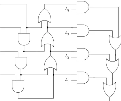
p s( ₃) p s( ₂) p s( ₁) p s( ₀) L₄ L₁ L₂ L₃

Figure 2: Circuit encoding for the LTL formulaFGpfork= 4

p p p p p p q q q q p q q q q q q p p p p p p p p p p q q q q q q q q q q p p p p p p p p p p p p p

Figure 3: Non-linear number of cubes in the translation ofG(r → (pUq)) fork = 4

Without sharing the formula is obviously cubic ink. Let us focus on the LTL part, the big underlined disjunction overl = 1, . . . , k. A first level of sharing can be obtained by associating the inner conjunction to the right, resulting in a quadratic DAG representation. Using the same general idea, the inner disjunction can be associated to the left. The overall size becomes linear. As an example see the circuit in Fig. 2 fork = 4. It can still be further optimised by applyinga∨(a∧b)≡a, which essentially results in removing the middle column of or-gates. However, as has been noted in [4], using associativity in synthesis is difficult and in general does not avoid the worst case, which is at least cubic.

As an example for the non-linear behaviour of the original translation [2] consider the (E)LTL formulaG(r→(pUq)). In the result of the translation we focus on propositional subformulas, which represent the translation of the inner temporal operator at all positionsi = 0, . . . , k −1and all loop starts

l = 1, . . . , k. Following Def. 13 in [2] these formulas are sum of product forms. Each product is a cube of the predicatespandq at various states. In Fig. 3 we list all cubes that occur as subformulas fork = 4. Each cube is represented by one row of the four matrices in Fig. 3. Each of the matrices collects those cubes where q holds at the same position resp. in the same state.

The number of cubes is at least quadratic ink. For each positionj where

q holds, thepsequences can be shared. Therefore an upper bound on the overall size isO(k3_{)and notO(k}4_{). The exact size is hard to calculate, but} with Ω(k2_{) different cubes in the example, the size has a quadratic lower} bound as well.

2.1 LTL

An LTL formulaϕis defined over a set of atomic propositionsAP. An LTL formula has the following syntax:

1. ψ ∈AP is an LTL formula.

2. Ifψandϕare LTL formulae then so are¬ψ,Xψ,ψUϕ,ψRϕ,ψ∧ϕ, andψ∨ϕ.

The operators are the next-time operatorX, the until operatorU, and its dual the release operatorR.

Each formula defines a set of infinite words (models) over2AP_{. Letπ ∈}

(2AP)ω be an infinite word. We denote the suffix of a wordπ = σ0σ1σ2. . . by πi _{= σ}

iσi+1σi+2. . . where σi ∈ 2AP, and πi denotes the prefix πi =

σ0σ1. . . σi. When a formulaψdefines a wordπat timeithis is denotedπi |=

ψ. The set of infinite words defined by a formulaψis{π ∈(2AP)ω |π|=ψ}. The relation ’|=’ is inductively defined in the following way.

πi |=ψ ⇔ ψ ∈σiforψ ∈AP.

πi |=¬ψ ⇔ π6|=ψ.

πi _{|=ψ∨ϕ ⇔ π}i _|=ψorπi _|=ϕ.

πi |=ψ∧ϕ ⇔ πi |=ψandπi |=ϕ. πi |=Xψ ⇔ πi+1 |=ψ.

πi _{|=ψUϕ ⇔ ∃n≥isuch thatπ}n_|=ϕandπj _{|=ψ for alli≤j < n.}

πi |=ψRϕ ⇔ ∀n≥i, πn |=ϕorπj |=ψfor somei≤j < n.

If π0 _{|= ψ we simply write π |= ψ. This presentation of the semantics is} intentionally redundant. The additional operators allow us to transform any formula to apositive normal form. Formulas in positive normal form have negations only in front of atomic propositions. Using the dualitiesψUϕ ≡ ¬(¬ψR¬ϕ),¬Xψ ≡X¬ψ and De Morgan’s law, any formula can be trans-formed without blowup to positive normal form by pushing in the negations. All formulas considered in this paper are assumed to be in positive normal form. We also make use of the standard abbreviations> ≡p∨¬pfor some ar-bitraryp∈AP,⊥ ≡ ¬>,Fψ ≡ >Uψ(’finally’), andGψ ≡ ⊥Rψ ≡ ¬F¬ψ

(’globally’).

A formula holds in a Kripke structure if all paths of the Kripke structure are accepted by the formula. Formally, a Kripke structure is a tuple M = (S, T, s0, L), where S is a set of states, T ⊆ S ×S the transition relation,

s0 ∈ S the initial state, and L : S → 2AP a function labelling all states with atomic propositions. We require that the transition relation is total. A path of the Kripke structure is a sequence of states ξ = s0s1s2. . . where

s0 is the initial state and for all i ≥ 0 we have that (si, si+1) ∈ T. The corresponding wordπ of a path ξ = s0s1s2. . .is π = L(s0)L(s1)L(s2). . .. 4 2 BOUNDED MODEL CHECKING

We writeM |=ψ, if for all pathsξ=s0s1s2. . .ofM the corresponding word

πis defined byψ, i.e.π |=ψ.

Bounded model checking uses abounded semantics of LTL which safely under approximates the normal semantics. It allows us to use a bounded pre-fixπk =s0s1. . . skof an infinite pathπto check the formula. The semantics

does a case split depending on if the infinite π is a k-loop or not. Biere et al. [2] have shown that if a formulaψ is true in the bounded semantics, de-notedπ |=k ψ, this implies that π |= ψ. The definition below assumes the

formula is in positive normal form.

Definition 1 ([2, 9]) Given an infinite path πand boundk ∈ N, a formula

ψholds in a pathπ with boundkiffπ|=0

kψ where π|=i_k p ⇔ p∈siforp∈AP π|=i_k ¬p ⇔ p6∈siforp∈AP π|=i k ψ1∧ψ2 ⇔ π|=ki ψ1andπ|=ikψ2 π|=i_k ψ1∨ψ2 ⇔ π|=ikψ1orπ|=ikψ2 π|=i_k Xψ ⇔ ( π|=i_k+1ψ πis ak-loop π|=i_k+1ψ∧(i < k) otherwise π|=i k ψ1Uψ2 ⇔ ( ∃j ≥i:π|=j_k ψ2∧ ∀n, i≤n < j:π|=nk ψ1 k-loop ∃j, i≤j≤k:π|=j_k ψ2∧ ∀n, i≤n < j:π|=nk ψ1 otherwise π|=i_k ψ1Rψ2 ⇔ ( ∀j ≥i:π6|=j_k ψ2 =⇒ ∃n, i≤n < j:π|=nk ψ1 k-loop ∃j, i≤j≤k:π|=j_k ψ1∧ ∀n, i≤n≤j:π|=nk ψ2 otherwise 3 A NEW TRANSLATION

Our new translation takes advantage of the fact that for lasso-shaped Kripke structures the semantics of LTL and CTL coincide [15, 19]. The intuition is that when each state has one successor (i.e. the path is lasso-shaped) the se-mantics of the path quantifiersAandEof CTL agree. An LTL formula can therefore be evaluated in a lasso-shaped Kripke structure by a CTL model checker by prefixing each temporal operator by an E path quantifier [19], which results in a CTL formula.1 _{We can thus use the fixpoint} characterisa-tion of CTL model checking as a starting point for our translacharacterisa-tion. The new translation also separates the concern of if the path has a(k, l)-loop from the semantics to an independent part of the translation.

The intuition behind our translation is the following. Following [2], we generate a propositional formula which generates all paths of length k. A part is added to the translation which makes a choice between the following possibilities. Either (a) there is no loop, or (b) there is a loop, i.e. a state

sl−1 such that sk = sl−1 for some index1 ≤ l ≤ k. The choice and addi-tional constraints under which the choice can be made are implemented as follows. Fresh variablesli, which do not depend on the state variables in any

way, are introduced with appropriate constraints such that if li is true then

si−1 =sk. We allow at most oneli to be true in a satisfying truth assignment.

This results in a lasso-shaped Kripke structure or a simple finite path if noliis

1_{Naturally, we could also use theApath quantifier.}

true. Allowing simple finite paths is an optimisation and does not affect cor-rectness, but can in some cases (formulas with safety-counterexamples) result in shorter counterexamples. Model checking is accomplished by generating propositional formulas to evaluate the greatest and least fixpoints as required by the implicit CTL formula.

Let M be the Kripke structure of the system and T(s, s0) the symbolic transition relation. We consider an unrolling of states s0s1. . . sk. Each si

is a vector of state variables. The unrolling is obtained by equation (1). We require that the Kripke structure is lasso-shaped or a finite path. The variables

li can seen as selecting one (or possibly none) of the possible (k, l)-loops.

This is accomplished by the following constraints.

|[LoopConstraints]|_k ⇔ Loop_k∧AtMostOnek Loopk ⇔ Vk i=1(li ⇒(si−1 =sk)) AtMostOnek ⇔ Vk i=1(SmallerExistsi ⇒ ¬li) SmallerExists1 ⇔ ⊥

SmallerExistsi+1 ⇔ SmallerExistsi∨li, where 0< i≤k

In contrast to [2], our definitions also allow the no loop case even if the path has a(k, l)-loop.

The until operator E(ψ1Uψ2) can be evaluated by computing the least fixed pointE(ψ1Uψ2) = µZ.ψ2 ∨(ψ1 ∧EXZ) (see e.g. [5]) while the re-lease operatorE(ψ1Rψ2)can be evaluated by computing the greatest fixpoint

E(ψ1Rψ2) =νZ.ψ2∧(ψ1∨EXZ). The fixpoints are evaluated by first com-puting an approximationhh·ii_i for each state and subformula. After this the results of the approximation are used to compute the final result|[·]|_i. We evaluate the fixpoints forsi where0≤i≤k+ 1. The last casek+ 1is added

to make the connections to fixpoints easier to see from the translation.

:= i≤k i=k+ 1 |[p]|_i pi Wk j=1(lj ∧pj) |[¬p]|_i ¬pi Wk j=1(lj ∧ ¬pj) |[Xψ]|_i |[ψ]|_i+1 Wk j=1 lj ∧ |[ψ]|j+1 |[ψUϕ]|_i |[ϕ]|_i∨ |[ψ]|_i∧ |[ψUϕ]|_i+1 Wk j=1 lj ∧ hhψUϕii_j |[ψRϕ]|_i |[ϕ]|_i∧ |[ψ]|_i∨ |[ψRϕ]|_i+1 Wk j=1 lj ∧ hhψRϕii_j hhψUϕii_i |[ϕ]|_i∨ |[ψ]|_i∧ hhψUϕii_i+1 ⊥ hhψRϕii_i |[ϕ]|_i∧ |[ψ]|_i∨ hhψRϕii_i+1 >

The auxiliary translation hh·ii which computes the approximations for the fixpoints is defined in the last two rows.

Let us consider the caseψ =ψ1Rψ2. We initialisehhψii_k+1to true since we are approximating a greatest fixpoint. When 0 ≤ i ≤ k, the auxili-ary translation hhψii_i is the normal fixpoint definition of the release oper-ator. The computed approximation of the fixpointhhψiiis used to initialise

|[ψ]|_k+1 with the value ofhhψii_l (this value is in fact exact), the successor of

sk, when we are dealing with a(k, l)-loop. Finally,|[ψ]|i, where0≤ i ≤ k,

computes the accurate values for each statesi, again using the standard

fix-point characterisation of release.

Given a Kripke structureM, an LTL formulaψ, and a boundk, the com-plete encoding as a propositional formula is given by|[M, ψ, k]|.

|[M, ψ, k]|=|[M]|_k∧ |[LoopConstraints]|_k∧ |[ψ]|₀

Theorem 1 Given a finite Kripke structureM, a boundk ∈ _Nand an LTL formulaψ,M has a pathπwithπ|=kψ iff|[M, ψ, k]|is satisfiable.

Proof:

The proof sketch follows the argument at the beginning of this Section. For both directions we can assume thatπ is given and is a path of M. Further assume thatπis a(k, l)loop. The other case is obvious from the definitions. The bounded semantics on a(k, l) loop coincides with the unbounded se-mantics. What remains to be proven is that the LTL part of the translation when partially instantiated withπis satisfiable iffπ|=ψ.

Instead of checking whether ψ holds along π we check the correspond-ing CTL formulaψ0 onπ interpreted as a Kripke structure itself. The CTL formulaψ0is obtained fromψ by prefixing every temporal operator with the existential path quantifierE. The ECTL formulaψ0 can be translated into an alternation free formula of the modal mu-calculus, which in turn can be transformed into a set of mutual recursive boolean equations with fixpoint semantics as in [7]. The event-driven linear fix point algorithm of [7] is then reformulated symbolically as a non-recursive boolean equation system, which

is equivalent to our definition of|[·]|. ut

As in Theorem 9 of [2] we can lift our Theorem 1 to the unbounded semantics. An upper bound onk would then be of the order O(|ψ| · |M| ·

2|ψ|_{). This is easy to show using the automata-theoretic approach to model} checking [21, 16, 20]. However, our main result is the following:

Theorem 2 |[M, ψ, k]| seen as Boolean circuit is linear in |T|, |ψ|, and k. More precisely, it is of the sizeO(|I|+ ((|T|+|ψ|)·k)), where|I|and |T|

are the sizes of the initial state predicate and the transition relation seen as Boolean circuits, respectively.2

Proof:

Obviously the translation ofLoopConstraints_k is linear w.r.t.k, since both

Loop_kandAtMostOnekloop once overk. We will argue the linearity of|[·]|

using the until-case, as it is the most complex. For each 0 ≤ i ≤ k, the translation adds a constant number of constraints. The casei=k+ 1addsk

constraints that refer tohhUii_i. This does not result in a quadratic formula, even thoughhhUii_i is linear, becausehhUii_ican clearly be shared between the constraints. Linearity ofhhUii_i is obvious as only a constant number of

constraints are added for each0≤i≤k+ 1. ut

2_{This bound applies to both to the number of gates and the number of wire connections}

between the gates of the Boolean circuit in question.

3.1 Optimising the Translation

A simple way to optimise the translation is to introduce special translations for certain derived operators. We have developed special translations for

Gψ,Fψ,GFψ and FGψ. These formulas have similarities which can also be seen in the way they share translations in the casei = k + 1. Note that the translations of |[GFψ]|_i and |[FGψ]|_i are only dependent on the case

i = k+ 1 since the semantics of the formulas only places requirements on states inside the loop.

:= i≤k i=k+ 1 |[Gψ]|_i |[ϕ]|_i∧ |[Gψ]|_i+1 Wk j=1 lj ∧ hhGψii_j |[Fψ]|_i |[ϕ]|_i∨ |[Fψ]|_i+1 Wk j=1 lj∧ hhFψiij |[GFψ]|_i |[GFψ]|_k+1 Wk j=1 lj∧ hhFψii_j |[FGψ]|_i |[FGψ]|_k+1 Wk j=1 lj ∧ hhGψii_j hhGψii_i |[ϕ]|_i∧ hhGψii_i+1 > hhFψii_i |[ϕ]|_i∨ hhFψii_i+1 ⊥

The translations for the above derived operators can be further optimised at the cost of introducingk+ 1additional variables. However, the new variables are functionally dependent on the variablesli and are shared by all

subfor-mulas using them. The variablesInLoop_j, where0< j ≤k, express the fact that the statesj is in the loop selected by the li variables. Additionally, we

introduce the variableLoopExists which is true iff the path s0s1. . . sk has

a(k, l)-loop. In other words,LoopExists is false iffπk is treated as a simple

path without a loop. This is encoded by the following definitions.

InLoop_i+1 ⇔ InLoop_i∨li+1 for 0< i < k

InLoop₁ ⇔ l1

LoopExists ⇔ InLoopk

With theInLoop_ivariables we can eliminate the need for the auxiliary trans-lationhh·iifor the derived operators. This simplifies the translation in most cases. The change in the translation is small as only the case i = k + 1 changes. Sharing also occurs between the translation for different operators as the translations forGψ andFGψ, and forFψ andGFψ are the same.

|[Gψ]|_k+1 =|[FGψ]|_k+1 = LoopExists∧Vk

i=1(¬InLoopi∨ |[ψ]|i) |[Fψ]|_k+1 =|[GFψ]|_k+1 = Wk

i=1(InLoopi∧ |[ψ]|i)

3.2 Fairness

In many cases we wish to restrict the possible executions of the system to dis-allow executions which are unrealistic or impossible in the physical system. The standard way is to add fairness constraints to the model in order to only obtain interesting counterexamples.

There are a few well-known notions of fairness. Justice(weak fairness) re-quires that certain conditions are true infinitely often. Compassion (strong fairness) requires that if certain conditions are true infinitely often then cer-tain other conditions must also hold infinitely often.

Let {J1, . . . , Jj} be a set of Boolean predicates over the state variables

which define the conditions that should be true infinitely often. Justice can then be expressed as the LTL formula

J =

j

^

i=1

GFJi.

Similarly, compassion can be expressed as an LTL formula. A set of pairs of Boolean predicates{(L1, U1), . . . ,(Lc, Uc)}over the state variables define

the compassion sets. Compassion is defined by the formula

C =

c

^

i=1

(GFLi ⇒GFUi).

We include the fairness constraints in the specification. Thus, instead of model checking the formulaψ, we check the formulaJ ∧ C →ψ. Since our propositional encoding of LTL formulas is linear, our overhead for handling fairness is linear in the number of fairness constraints.

4 RELATED WORK

This work can be seen as a continuation of the work done in [11]. There the bounded model checking problem for LTL is translated into the problem of finding a stable model of a normal logic program (another NP-complete problem, see references in [11]) of essentially (modulo a constant) the same size as the translation presented here. The main differences to that work are the following. (i) The translation of [11] uses the close correspondence between the stable model semantics with the notion of a least fixpoint of a set of Boolean equations. The “formula variable dependency graphs” of the translation of [11] are in fact cyclic, while in this work they are acyclic. See-ing the translation of [11] as a propositional formula would result in a transla-tion which isnotsound. By using the correspondence between least fixpoints and stable models the translation for until and release formulas in [11] do not require the auxiliary translationshh·ii. Thus the translation of [11] had to be significantly changed in order to use SAT. Additionally, the best known automatic translation of the stable model problem to SAT is non-linear [13]. (ii) The translation in [11] employs a different system modelling formalism, which allows for partial order semantics based optimisations. (iii) Moreover, the translation in [11] also allows for deadlocking systems with LTL inter-preted over finite paths in the case of a deadlock, a feature left for further work in this paper. (iv) Finally, the implementation presented in this work is new, and based on the NuSMV2 [3] system.

Others have also considered the problem of improving the BMC encod-ing [4, 9, 6]. Cimatti et al. [4] analyse the original encodencod-ing [2] and suggest

several optimisations. For instance, they propose a linear encoding for for-mulas of the formGFp. Their translation is, however, not linear in general. Frisch et al. [9] approach the translation problem by using a normal form of LTL and take advantage of the properties of the normal form. Their pro-cedure modifies the original model and is similar to symbolic tableau-style approaches for LTL model checking. According to their experiments their approach produces smaller encodings than [4]. However, their encoding is also non-linear in the general case. The non-linearity occurs at least in those cases when model checking a formula ψ such that after converting ¬ψ to positive normal form it contains until or finally operators. Closest to their method is the so calledsemantic translation for BMC [8, 6]. The method follows closely the standard automata theoretic approach to model check-ing and creates a product systemM×B¬ψ, whereB¬ψis a Büchi automaton

representing the negation of the property. The existence of a counterexample is demonstrated by finding a fair loop in the product system. Since only fair loops are accepted the method does not find counterexamples without a loop. This is the main drawback of the method, and is something which could be improved upon in the future. The greatest advantage of the method is that it can leverage the significant amount of research which has been invested in improving the efficiency of LTL to Büchi automata translators. The transla-tion results in a linear number of variables but a quadratic number clauses because of the way fairness is handled. Naturally, the semantic translation could also be improved to linear by e.g. using the translation presented in this work or that of [4]. Furthermore, the approach used in the experiments of [6] results in a translation which is exponential in the LTL formula length as the Wring system used produces explicit state Büchi automata instead of symbolic ones.

Many researchers have also investigated improving SAT solver efficiency. Strichman [18] uses the special properties of the formula Gp to improve solver efficiency of BMC problems. As most safety properties can be reduced to checking invariants, the methods introduced are applicable for safety prop-erties in general. Gupta et al. [10] use BDD model checking runs for training the solvers to achieve better performance.

5 EXPERIMENTS

In order to evaluate the practical impact of our new linear translation we have performed two series of experiments. The first series of experiments evalu-ates the performance of the encoding on random formulae in small random Kripke structures, while the second series of experiments benchmarks the performance on real-life examples. Our implementation is compared against two bounded LTL model checking algorithms. Firstly we compare against the standard NuSMV encoding [3], which includes many of the optimisa-tions of [4]. We also compare against the encoding of [9] which we will call Fixpoint. We do not compare against the SNF encoding also available in [9] since generally the Fixpoint encoding performs better than SNF. In order to make all other implementation differences as small as possible, all of the en-codings were benchmarked on top of the NuSMV version of D. Sheridan [9] 10 5 EXPERIMENTS

(obtained from his homepage on 18th of March 2004) which contains sev-eral BMC related optimisations not included in the standard NuSMV 2.1 distribution. We expect that benchmarking the implementations on top of NuSMV 2.1 would result in larger running times for all the implementations in question at least in the random Kripke structures benchmark. It should be noted that the compact CNF conversion [12] option of the tool was disabled. In the first series of experiments we generated small random Kripke struc-tures and random formulae using techniques from [19]. The experiments give us some sense of how the implementations scale when the bound or the size of the formula is increased. To demonstrate the cases where the non-linearity of the Fixpoint translation occurs we generated formulas¬ψ which in positive normal form contains a larger percentage of finally and until op-erators than other temporal opop-erators. For each formula size we generate 40 formulas, which we then model check by forcing the model checker to look for counterexamples which are of exactly the length specified by the bound. The random Kripke structures we use contain 30 states and one weak fairness constraint which holds in two randomly selected states. We measure the time used to solve the SAT instance and the number clauses and variables in the instance.

When benchmarking against NuSMV default translation we varied the size of the formula from 3 to 10. For each formula size we let the bound grow up tok = 30.

When benchmarking against Fixpoint translation we were able to increase both the bounds used and the formula sizes to better demonstrate the differ-ences between the two translations. We varied the size of the formula from 3 to 14. For each formula size we let the bound grow up tok = 50.

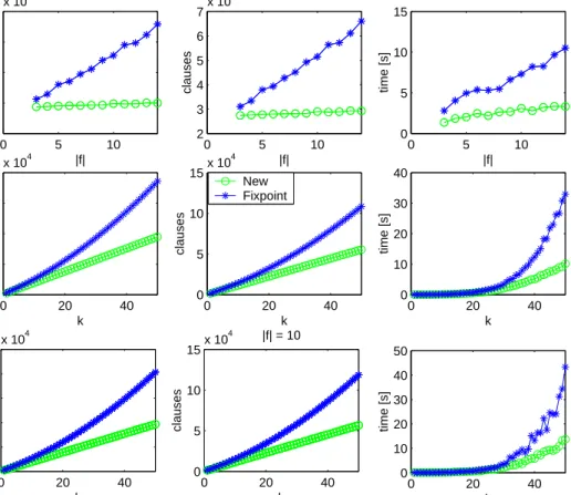
In Figures 4 and 5 there are nine plots in each figure which depict the res-ults from tests with random formulae of the new translation against NuSMV and Fixpoint, respectively. The three top plots show the average time, aver-age number of clauses, and averaver-age number of variables for each formula size over all bounds. In the second row the we have computed the same measures when averaged for each bound over all formula sizes. The last row shows the averages when the size of formula is fixed at ten. The plots clearly show the non-linearity of the competing translations [4, 9] with respect to the bound. Something the plots do not show is time for generating the problems. Our ex-perience is that the new implementation and Fixpoint generated the Boolean formulas almost instantaneously while for the NuSMV encoding there were cases where generation time dominated. In fact, a couple of NuSMV data points had to be omitted from the averages due to the fact that the generation of the SAT instance took several hours.

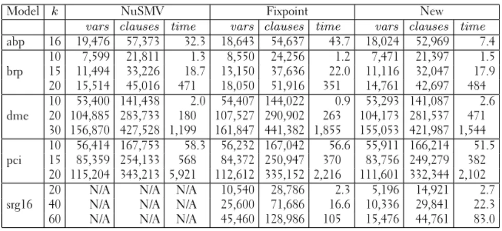
In the second series of experiments we used real-life examples. As specific-ations we favoured longer formulas since all implementspecific-ations can translate simple formulas linearly. The models we used were a model of the altern-ating bit protocol (abp), a distributed mutual exclusion algorithm (dme), a bounded resource protocol (brp), a model of a pci bus (pci), and a model of a 16-bit shift register (srg16). The results for the real-life examples are summarised in Table 1. We measured the number of variables, cumulat-ive number of clauses and the time used to verify formulas for the reported maximum bound. For the real-life examples, Fixpoint or the new translation

0 5 10 0.5 1 1.5x 10 4 |f| variables 0 5 10 1 2 3 4x 10 4 |f| clauses 0 5 10 0 1 2 3 |f| time [s] 0 10 20 30 0 1 2 3x 10 4 k variables 0 10 20 30 0 2 4 6 8x 10 4 k clauses 0 10 20 30 0 2 4 6 8 k time [s] 0 10 20 30 0 1 2 3 4x 10 4 k variables 0 10 20 30 0 5 10 15x 10 4 _{|f| = 10} k clauses 0 10 20 30 0 5 10 15 k time [s] NuSMV New

Figure 4: Plots for NuSMV and New, averages over random formulae

0 5 10 0.5 1 1.5 2 2.5x 10 4 |f| variables 0 5 10 2 3 4 5 6 7x 10 4 |f| clauses 0 5 10 0 5 10 15 |f| time [s] 0 20 40 0 1 2 3 4x 10 4 k variables 0 20 40 0 5 10 15x 10 4 k clauses 0 20 40 0 10 20 30 40 k time [s] 0 20 40 0 1 2 3 4 5x 10 4 k variables 0 20 40 0 5 10 15x 10 4 _{|f| = 10} k clauses 0 20 40 0 10 20 30 40 50 k time [s] New Fixpoint

Figure 5: Plots for Fixpoint and New, averages over random formulae

Table 1: Benchmarks

Model k NuSMV Fixpoint New

vars clauses time vars clauses time vars clauses time

abp 16 19,476 57,373 32.3 18,643 54,637 43.7 18,024 52,969 7.4 10 7,599 21,811 1.3 8,550 24,256 1.2 7,471 21,397 1.5 brp 15 11,494 33,226 18.7 13,150 37,636 22.0 11,116 32,047 17.9 20 15,514 45,016 471 18,050 51,916 351 14,761 42,697 484 10 53,400 141,438 2.0 54,407 144,022 0.9 53,293 141,087 2.6 dme 20 104,885 283,733 180 107,527 290,902 263 104,173 281,537 471 30 156,870 427,528 1,199 161,847 441,382 1,855 155,053 421,987 1,544 10 56,414 167,753 58.3 56,232 167,042 56.6 55,911 166,214 51.5 pci 15 85,359 254,133 568 84,372 250,947 370 83,756 249,279 382 20 115,204 343,213 5,921 112,612 335,152 2,216 111,601 332,344 2,102

20 N/A N/A N/A 10,540 28,786 2.3 5,196 14,921 2.7

srg16 40 N/A N/A N/A 25,600 71,686 16.6 10,336 29,841 22.3 60 N/A N/A N/A 45,460 128,986 105 15,476 44,761 83.0

are usually the fastest.

Our new translation is the most compact one in all cases. However, the differences are small as the model part of the translation dominates the trans-lation size. The shift register example (srg16) shows the strength of a linear translation. NuSMV could not managek = 20in a reasonable time while Fixpoint displays non-linear growth with respect tok.

All experiments were performed on a computer with an AMD Athlon XP 2000+ processor and 1 GiB of RAM using the SAT solver zChaff [17], ver-sion 2003.12.04.

5.1 Implementation

The translation can be straightforwardly implemented as a recursive proced-ure which does case analysis based on the translation. Implementation sim-plicity is, in our opinion, one of the main strengths of the new translation. The only implementation optimisation used was a simple cache, implemen-ted as a lookup table, for the values of|[·]|_i andhh·ii_i. This avoids a blow up in run time for certain formulas and speeds up the generation of the Boolean formula. All encoding optimisations mentioned in Sect. 3.1 have of course been implemented.

6 CONCLUSIONS

We have presented a translation of the bounded LTL model checking prob-lem to SAT which is linear in the bound and the size of the formula. The translation produces a linear number of variables and clauses in the resulting CNF.

Our benchmarks show that our new translation scales better both in size of the bound and the size of the formula than previous implementations [4, 9]. The translation remains linear in all cases. However, in some cases either the size of the formula or the bound must be made large before the benefit shows. One avenue of future work is to include some of the optimisations presented in [4] in order to the improve the performance of our translation for short formulas and small bounds.

Other avenues of future work also exist. One fairly straightforward gen-eralisation of our translation is the ability to handle deadlocking executions. This could probably be done in a manner similar to [11]. Another inter-esting topic is generalising our translation to include past temporal logic as the translation of [1]. The presented translation could also benefit from spe-cific SAT solver optimisations. When the translation is seen as producing Boolean circuits, all of the circuits are monotonic if theInLoopvariables and state variables (and their negated versions) are given as inputs. A solver (also CNF-based) could be optimised to take advantage of this.

Acknowledgements

We gratefully acknowledge the financial support of Helsinki Graduate School in Computer Science (HeCSE), the Academy of Finland (project 53695 and grant for research work abroad), the Nokia Foundation, FET pro-ject ADVANCE contract No IST-1999-29082, and EPSRC grant 93346/01 (An Automata Theoretic Approach to Software Model Checking). This work has also been sponsored by the CALCULEMUS! IHP-RTN EC project, con-tract code HPRN-CT-2000-00102, and has thus benefited of the financial contribution of the Commission through the IHP programme.

We would also like to thank D. Sheridan for sharing his NuSMV imple-mentation with us.

REFERENCES

[1] M. Benedetti and A. Cimatti. Bounded model checking for past LTL. In Tools and Algorithms for Construction and Analysis of Systems (TACAS’2003), volume 2619 ofLNCS, pages 18–33. Springer, 2003. [2] A. Biere, A. Cimatti, E. Clarke, and Y. Zhu. Symbolic model

check-ing without BDDs. InTools and Algorithms for the Constructions and Analysis of Systems (TACAS’99), volume 1579 of LNCS, pages 193– 207. Springer, 1999.

[3] A. Cimatti, E. Clarke, E. Giunchiglia, F. Giunchiglia, M. Pistore, Marco Roveri, R. Sebastiani, and Armando Tacchella. NuSMV 2: An opensource tool for symbolic model checking. In Computer Aided Verification (CAV’2002), volume 2404 ofLNCS, pages 359–364. Springer, 2002.

[4] A. Cimatti, M. Pistore, M. Roveri, and R. Sebastiani. Improving the encoding of LTL model checking into SAT. In Verification, Model Checking, and Abstract Interpretation (VMCAI’2002), volume 2294 of LNCS, pages 196–207. Springer, 2002.

[5] E. Clarke, O. Grumberg, and D. Peled. Model Checking. The MIT Press, 1999.

[6] E. Clarke, D. Kroenig, J. Oukanine, and O. Strichman. Completeness and complexity of bounded model checking. In Verification, Model 14 REFERENCES

Checking, and Abstract Interpretation (VMCAI’2004), volume 2937 of LNCS, pages 85–96. Springer, 2004.

[7] R. Cleaveland and B. Steffen. A linear-time model-checking algorithm for the alternation-free modal mu-calculus. Formal Methods in System Desing, 2(2):121–147, 1993.

[8] L. de Moura, H. Rueß, and M. Sorea. Lazy theorem proving for bounded model checking. In Conference on Automated Deduction (CADE’02), volume 2392 ofLNCS, pages 438–455. Springer, 2002. [9] A. Frisch, D. Sheridan, and T. Walsh. A fixpoint encoding for bounded

model checking. InFormal Methods in Computer-Aided Design (FM-CAD’2002), volume 2517 ofLNCS, pages 238–255. Springer, 2002. [10] A. Gupta, M. Ganai, C. Wang, Z. Yang, and P. Ashar. Learning from

BDDs in SAT-based bounded model checking. InProceedings of the 40th Conference on Design Automation, pages 824–829. IEEE, 2003. [11] K. Heljanko and I. Niemelä. Bounded LTL model checking with stable

models. Theory and Practice of Logic Programming, 3(4–5):519–550, 2003.

[12] P. Jackson and D. Sheridan. The optimality of a fast CNF conversion and its use with SAT. Technical Report APES-82-2004, APES Research Group, March 2004. Available from http://www.dcs.st-and.ac.

uk/~apes/apesreports.html.

[13] T. Janhunen. A counter-based approach to translating logic programs into set of clauses. In Proceedings of the 2nd International Workshop on Answer Set Programming (ASP’03), volume 78, pages 166–180. Sun SITE Central Europe (CEUR), 2003.

[14] D. Kroenig and O. Strichman. Efficient computation of recurrence diameters. In Verification, Model Checking, and Abstract Interpreta-tion (VMCAI’2003), volume 2575 ofLNCS, pages 298–309. Springer, 2003.

[15] O. Kupferman and M.Y. Vardi. Model checking of safety properties. Formal Methods in System Design, 19(3):291–314, 2001.

[16] R.P. Kurshan.Computer-Aided Verification of Coordinating Processes: The Automata-Theoretic Approach. Princeton University Press, 1994. [17] M. Moskewicz, C. Madigan, Y. Zhao, L.Zhang, and S. Malik. Chaff:

Engineering an efficient SAT solver. InProceedings of the 38th Design Automation Conference, 2001.

[18] O. Strichman. Accelerating bounded model checking of safety proper-ties. Formal Methods in System Design, 24(1):5–24, 2004.

[19] H. Tauriainen and K. Heljanko. Testing LTL formula translation into Büchi automata. STTT - International Journal on Software Tools for Technology Transfer, 4(1):57–70, 2002.

[20] M.Y. Vardi. An automata-theoretic approach to linear temporal logic. InLogics for Concurrency: Structure versus Automata, volume 1043 of LNCS, pages 238–266. Springer, 1996.

[21] M.Y. Vardi and P. Wolper. An automata-theoretic approach to auto-matic program verification. InProceedings of the First Symposium on Logic in Computer Science, pages 322–331, Cambridge, 1986.

HELSINKI UNIVERSITY OF TECHNOLOGY LABORATORY FOR THEORETICAL COMPUTER SCIENCE RESEARCH REPORTS

HUT-TCS-A79 Heikki Tauriainen

Nested Emptiness Search for Generalized Bu¨chi Automata. July 2003.

HUT-TCS-A80 Tommi Junttila

On the Symmetry Reduction Method for Petri Nets and Similar Formalisms. September 2003.

HUT-TCS-A81 Marko Ma¨kela¨

Efficient Computer-Aided Verification of Parallel and Distributed Software Systems. November 2003.

HUT-TCS-A82 Tomi Janhunen

Translatability and Intranslatability Results for Certain Classes of Logic Programs. November 2003.

HUT-TCS-A83 Heikki Tauriainen

On Translating Linear Temporal Logic into Alternating and Nondeterministic Automata. December 2003.

HUT-TCS-A84 Johan Walle´n

On the Differential and Linear Properties of Addition. December 2003.

HUT-TCS-A85 Emilia Oikarinen

Testing the Equivalence of Disjunctive Logic Programs. December 2003.

HUT-TCS-A86 Tommi Syrja¨nen

Logic Programming with Cardinality Constraints. December 2003.

HUT-TCS-A87 Harri Haanpa¨a¨, Patric R. J. O¨ sterga˚rd

Sets in Abelian Groups with Distinct Sums of Pairs. February 2004.

HUT-TCS-A88 Harri Haanpa¨a¨

Minimum Sum and Difference Covers of Abelian Groups. February 2004.

HUT-TCS-A89 Harri Haanpa¨a¨

Constructing Certain Combinatorial Structures by Computational Methods. February 2004.

HUT-TCS-A90 Matti Ja¨rvisalo

Proof Complexity of Cut-Based Tableaux for Boolean Circuit Satisfiability Checking. March 2004.

HUT-TCS-A91 Mikko Sa¨rela¨

Measuring the Effects of Mobility on Reactive Ad Hoc Routing Protocols. May 2004.

HUT-TCS-A92 Timo Latvala, Armin Biere, Keijo Heljanko, Tommi Junttila Simple Bounded LTL Model Checking. July 2004.

ISBN 951-22-7223-7 ISSN 1457-7615