Dissertation
zur Erlangung des akademischen Grades Doktoringenieur (Dr.-Ing.)
vorgelegt an der
Technischen Universit¨at Dresden Fakult¨at Informatik
eingereicht von
Dipl.-Inf. Konrad Voigt
geboren am 21. Januar 1981 in Berlin
Gutachter:
Prof. Dr. rer. nat. habil. Uwe Aßmann (Technische Universität Dresden) Prof. Dr. Jorge Cardoso (Universidade de Coimbra, PT)
Tag der Verteidigung: Dresden, den 2. November 2011
Data integration has been, and still is, a challenge for applications process-ing multiple heterogeneous data sources. Across the domains of schemas, ontologies, and metamodels, this imposes the need for mapping specifica-tions, i.e. the task of discovering semantic correspondences between ele-ments. Support for the development of such mappings has been researched, producing matching systems that automatically propose mapping sugges-tions.
However, especially in the context of metamodel matching the result quality of state of the art matching techniques leaves room for improvement. Although the traditional approach of pair-wise element comparison works on smaller data sets, its quadratic complexity leads to poor runtime and memory performance and eventually to the inability to match, when applied on real-world data.
The work presented in this thesis seeks to address these shortcomings. Thereby, we take advantage of the graph structure of metamodels. Conse-quently, we derive a planar graph edit distance as metamodel similarity metric and mining-based matching to make use of redundant information. We also propose a planar graph-based partitioning to cope with large-scale matching. These techniques are then evaluated using real-world mappings from SAP business integration scenarios and the MDA community. The re-sults demonstrate improvement in quality and managed runtime and mem-ory consumption for large-scale metamodel matching.
This dissertation was conducted at SAP Research Dresden directed by Dr. Gregor Hackenbroich. I am grateful to SAP Research for financing this work through a pre-doctoral position.
Further, I want to express my gratitude to my advisor Prof. Uwe Aßmann as well as to Prof. Jorge Cardoso and Prof. Alexander Schill who agreed to be my co-advisors. I thank my supervisor Uwe Aßmann for giving me the opportunity to work on this interesting and challenging topic and for all the advises he gave me and Prof. Alexander Schill for constructive comments on this work. I owe a great debt to Prof. Jorge Cardoso, whom I had the pleasure to work with. Jorge has been the kind of mentor to me who all young researchers should have.
I am grateful to Petko Ivanov, Thomas Heinze, Peter Mucha, and Philipp Simon. It was very motivating to discuss with them and the thesis benefited a lot from their contributions. A big thanks to you students, without you this thesis would have been impossible.
Further, I would like to thank the people from the TU Dresden and SAP Research who helped me with their input and discussions. Special thanks go to the ones commenting on my work: Eldad Louw for his perfect En-glish and joy, Dr. Kay Kadner for his support in the TEXO project and magic moments, Eric Peukert for valuable discussions and expert knowledge ex-change, Birgit Grammel for reminding me of myself and sharing some of the PhD agonies, Dr. Andreas Rummler for the mentoring, Dr. Roger Kilian-Kehr for critical thoughts, Dr. Karin Fetzer for comments on short notice, Arne for physical and psychological work-outs, and Daniel Michulke for regular lunch-meetings. I am grateful to Dr. Gregor Hackenbroich for his support, his valuable and precise comments, and for allowing me to continue my work at SAP Research, and I would also like to thank Annette Fiebig who supported me not only in administrative issues.
I also would like to thank my friends for tolerating and enduring my absence and lust for work. Thank you for still knowing me. Finally, I want to thank my family for encouragement and enjoyable moments.
And thank you Karen not only for reading countless versions of my thesis and commenting each of them thoroughly but also thank you for all your love and trust in me. Thank you.
1 Introduction 1
1.1 Quality Problem in Matching . . . 3
1.2 Scalability Problem in Matching . . . 4
1.3 Research Questions and Contributions . . . 4
1.4 Thesis Outline . . . 7 2 Background 9 2.1 Metamodel Matching . . . 9 2.1.1 Metamodel . . . 9 2.1.2 Matching . . . 11 2.2 Graph Theory . . . 19 2.2.1 Definitions . . . 19 2.2.2 Metamodel representation . . . 20 2.2.3 Graph properties . . . 24 2.2.4 Graph matching . . . 28 2.2.5 Graph mining . . . 30
2.2.6 Graph partitioning and clustering . . . 31
2.3 Summary . . . 33
3 Problem Analysis 35 3.1 Motivating Example . . . 35
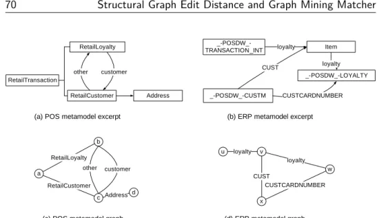
3.1.1 Retail scenario description . . . 35
3.1.2 ERP and POS metamodels . . . 37
3.1.3 Data integration problems . . . 38
3.2 Problem Analysis . . . 40
3.2.1 Problems and scope . . . 40
3.2.2 Objectives . . . 44 3.2.3 Requirements . . . 45 3.2.4 Approach . . . 46 3.2.5 Research question . . . 48 3.3 Summary . . . 48 iii
4.1.1 Schema matching . . . 52 4.1.2 Ontology matching . . . 53 4.1.3 Metamodel matching . . . 54 4.2 Matching Quality . . . 56 4.3 Matching Scalability . . . 58 4.4 Summary . . . 60
5 Structural Graph Edit Distance and Graph Mining Matcher 63 5.1 Planar Graph Edit Distance Matcher . . . 63
5.1.1 Analysis of graph matching algorithms . . . 64
5.1.2 Planar graph edit distance algorithm . . . 67
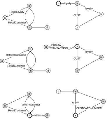
5.1.3 Example calculation . . . 70
5.1.4 Improvement by k-max degree partial seed matches . 72 5.2 Graph Mining Matcher . . . 73
5.2.1 Analysis of graph mining algorithms . . . 75
5.2.2 Graph model for mining based matching . . . 78
5.2.3 Design pattern matcher . . . 79
5.2.4 Redundancy matcher . . . 84
5.3 Summary . . . 89
6 Planar Graph-based Partitioning for Large-scale Matching 91 6.1 Partition-based Matching . . . 91
6.2 Planar Graph-based Partitioning . . . 93
6.2.1 Analysis of graph partitioning algorithms . . . 93
6.2.2 Planar Edge Separator based partitioning . . . 96
6.3 Assignment of Partitions for Matching . . . 102
6.3.1 Partition similarity . . . 103 6.3.2 Assignment algorithms . . . 104 6.3.3 Comparison . . . 109 6.4 Summary . . . 110 7 Evaluation 113 7.1 Evaluation strategy . . . 113
7.2 Evaluation framework: MatchBox . . . 115
7.2.1 Processing steps and architecture . . . 115
7.2.2 Matching techniques . . . 116
7.2.3 Parameters and configuration . . . 118
7.3 Evaluation Data Sets . . . 119
7.3.1 Data set metrics . . . 119
7.3.2 Enterprise service repository mappings . . . 121
7.3.3 ATL-zoo mappings . . . 126
7.5.1 Graph edit distance results . . . 135
7.5.2 Graph mining results . . . 141
7.5.3 Discussion . . . 144
7.6 Results for Graph-based Partitioning . . . 144
7.6.1 Partition size . . . 145 7.6.2 Partition assignment . . . 147 7.6.3 Summary . . . 151 7.7 Discussion of Results . . . 152 7.7.1 Applicability . . . 152 7.7.2 Limitations . . . 153 7.8 Summary . . . 154 8 Conclusion 157 8.1 Summary . . . 157
8.2 Conclusion and Contributions . . . 159
8.3 Recommendations for Data Model Development . . . 161
8.4 Further Work . . . 163
A Evaluation Data Import 167 A.1 ATL-zoo Data Import . . . 167
A.1.1 Import of metamodels . . . 168
A.1.2 Import of ATL-transformations . . . 168
A.2 ESR Data Import . . . 173
B MatchBox Architecture 175 B.1 Architecture . . . 175
B.2 Combination Methods . . . 175
Bibliography 179
Introduction
Data integration has been, and still is, a challenge for applications process-ing multiple heterogeneous data sources. Across the domains of schemas, ontologies, and metamodels this heterogeneity inevitably imposes the need for mapping specifications. Thereby, a mapping specification requires the task of creating semantic correspondences between elements to integrate multiple data sources.
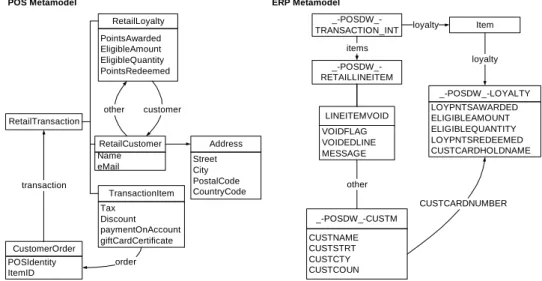
An industrial example for the integration of multiple data sources is given through the point of sale scenario [134], where data coming from several retail stores needs to be integrated in a central system. A retail store has cashiers processing sales using tills and a local system collecting all data. The data from the sales of products is sent to and aggregated in a central En-terprise Resource Planning (ERP) system [136]. Thereby, the central system and third-party systems of different stores naturally differ in their internal formats which may be defined using schemas, ontologies, or metamodels. To integrate the systems a mapping between the concepts of the third-party systems and the central ERP is needed. For instance, two different represen-tations for a purchase order or customer data have to be mapped onto each other. Support for the development of such mappings has been researched, producing matching systems that automatically propose mapping sugges-tions, e. g. in schema matching [126], ontology matching [33] and meta-model matching [98].
In the three matching domains most of the proposed systems claim an overall result of automatically finding nearly complete mappings, e. g. in [94, 25, 37, 38, 32]. These results are, however, only possible when run-ning on a limited data set. When applied on heterogeneous real-world data our evaluation demonstrates that established state of the art matching tech-niques show only approximately half of all possible mappings found. This observation has also been confirmed by the results of the ontology align-ment real-world task [32, 125]. Consequently, in this thesis we identified the challenge of (1)improving the quality of matching results.
The challenge of improving matching quality is not restricted to meta-model matching but also applies to schema and ontology matching. The three domains differ in the way data structures are defined. Schemas allow for a tree-based definition of elements and types. Ontologies and metamod-els follow a similar way with a graph-based structure, typed relations, and the notion of inheritance. The difference in structure also concerns matching which is either tree or graph-based utilizing the structures available.
In this thesis we concentrate on metamodel matching where the data is defined through metamodels using object-oriented concepts such as classes, attributes, references, etc. We focus on the area of metamodel matching and thus Model Driven Architecture (MDA) [118], since MDA constitutes an in-dustrial standard and specifies graph-based data models. This approach is justified by two reasons, first the field of metamodel matching is relatively unexplored and provides matching on typed graphs. Second, metamodels are increasingly applied in industry, for instance in SAP [4] throughout sev-eral products [135, 9, 143] leading to the necessity for improved matching systems. However, the concepts developed in this thesis are not restricted to metamodels but can also be applied to schema and ontology matching. The general applicability of our approach is demonstrated in our evaluation by applying our concepts to metamodels and schemas.
Besides the necessity of an improvement in matching quality another challenge is raised by an increase in size and complexity of schemas and metamodels in an enterprise context. As a consequence, the task of matching these large-scale schemas and metamodels for data integration purposes has surpassed the capabilities of most matching systems [125]. The traditional approach of pair-wise element comparison leads to quadratic complexity and thus runtime and memory issues. This results in the second challenge of (2)missing support for large-scale matching.
The goal of this thesis is to improve the result quality of metamodel matching in terms of correctness and completeness in the context of large-scale matching tasks. The main hypothesis of this thesis is that metamodel matching and matching in general can be improved by utilizing the graph structure of metamodels. This hypothesis is confirmed and validated us-ing real-world data, both from the domains of metamodels and business schemas.
In the following, we will discuss the problems of matching quality and scalability. Based on these problems we will state our research questions and corresponding hypotheses to conclude with our contributions. This introduc-tion is completed by outlining our thesis chapters.
1.1
Quality Problem in Matching
Metamodel matching aims at the calculation of mappings between two meta-models. These mappings should be presented to a user to support him in the task of mapping specification. Those mappings are finally used to integrate heterogeneous metamodels. Consequently, metamodel matching should re-duce the effort as well as errors in the process of mapping specification. Since the mappings calculated are intended to be used by a domain expert often in an enterprise context, it is essential that those mappings are, as far as possible, correct and complete. The correctness and completeness defines the quality of metamodel matching. If the mappings calculated show a low correctness and completeness, metamodel matching may even impose an additional burden to a user applying it. Therefore, quality is one of the main concerns of metamodel matching.
One reason for, on average, only about half of all mappings being found and being correct, is the insufficient amount of information contained in a metamodel, i. e. its expressiveness. A metamodel defines object-oriented structures and thus explicit information like packages, classes, relations, at-tributes, etc. But, a metamodel does not contain implicit information such as the meaning of terms, codes, preconditions, etc. This additional knowledge is typically only known to domain experts.
An improvement of quality can be achieved by taking additional infor-mation into account. This can be generic inforinfor-mation available, domain-specific knowledge, configurations or pre-processing and post-processing. For instance, the work of Garces [45] proposes a domain-specific language to incorporate external knowledge in matching processes. Some systems, e. g. [28], try to capture this additional knowledge in external representa-tions to improve matching quality. The additional knowledge is external, be-cause metamodels do not require a user to specify that information, thus it is not part of the metamodel. Another approach is to reuse existing mappings for instance by using transitivity for mapping calculation [23] or by cover-age analysis [132]. However, each of these approaches requires external or domain-specific knowledge which one cannot be taken for granted.
Another reason for deficits in matching quality is the existence of redun-dant information. This is due to the fact that one element may be mapped onto multiple occurrences of another, thus producing multiple mappings in-stead of one. This redundant information produces misleading mappings, which may present more incorrect mappings to a user.
To summarize we identified the problem of: (1) insufficient correctness and completeness of matching results.
1.2
Scalability Problem in Matching
The problem of scalability naturally arises in the context of large-scale data as confirmed by Rahm [125]. Especially in industry metamodels easily ex-ceed the size of 1,000 elements and may contain even more than 8,000 elements. For instance, the aforementioned point of sale scenario involves metamodels of such a size, because data about stores, customers, transac-tions, billing, etc. has to be stored [134]. Matching two metamodels with 8,000 elements each results in 64,000,000 comparisons to be made and stored in the memory for a combination. Even with state of the art ap-proaches this leads to issues of high memory consumption and a runtime overhead.
The memory and runtime problems result in an inacceptable system ap-plicability and usability. High memory consumption potentially leads to an unresponsive system and in the worst case to an abortion or crash of the matching system. The runtime problem becomes especially important in case of an interactive scenario. If a user wants to obtain metamodel match-ing results for a given matchmatch-ing task of two metamodels he typically wants to receive system feedback in seconds or better milliseconds. With large-scale metamodels the system response time increases quadratically to min-utes or even hours.
Only some systems tackle this problem by limiting the matching context with light-weight matching techniques [10]. However, these techniques re-duce the result quality significantly and do not tackle the memory problem for metamodels of arbitrary size. Another approach in the area of schema matching is to reduce the number of comparisons but not the schema size, e. g. in COMA++ [25] and aFlood [54]. These approaches apply a partition-ing on the input, splittpartition-ing it into smaller subparts and based on these parts define the comparisons to be made. However, the parts are not matched independently, thus the runtime is decreased but not the memory tion. Hence, the approaches do not solve the problems of memory consump-tion and unmatchable metamodels. In addiconsump-tion, the approaches [25, 54] are limited to schemas or ontologies, hence they are not easily applicable to metamodels. We derive the second cause problem of our thesis: a (2) missing support for matching metamodels of large-scale size.
1.3
Research Questions and Contributions
Our main objectives are to improve quality and increase scalability for meta-model matching. A solution using information additional to metameta-models is not a viable choice because this information is generally not available or requires an additional effort by a domain expert to produce. Therefore, we
focus on information inherent to metamodels, namely the structural graph information of a metamodel.
Structural graph information has been utilized for fix-point based simi-larity propagation in schema matching [107] but not for a comparison and similarity calculation solely based on structure. The reason lies in the sig-nificant computational complexity of the graph isomorphism problem. The calculation of an edge-preserving mapping between two graphs is known to belong to NP [47]. However, the complexity of (sub-)graph isomorphism calculation can be reduced by restricting a general graph structure to spe-cific graph classes that obey certain graph properties; an observation that will prove useful when investigating our research question:
Research question 1. ”How can metamodel graph structure be used to im-prove the correctness, completeness, runtime, and memory consumption of metamodel matching?”
The identification of general (sub-) graph isomorphism belongs to NP, therefore the complexity must be reduced. It is known that a restriction of the input graph to special classes of graphs reduces the complexity of the isomorphism calculation. The problem is to identify the type of classes which retain as much information as possible, thus the class which is the closest to the general graph.
A well-known class restricting the input are trees. Trees are used for path computations, indices, matching [162] etc. However, a tree represents only a smaller part of the original complete graph. Especially in the context of matching this imposes a drawback in terms of quality, because less context information is available for matching.
Another more general class of graphs, known since 1930, are planar graphs. Planar graphs are graphs which can be drawn in a plane without in-tersecting edges. They have been formally defined by Kuratowski’s Theorem [90]. These graphs allow for a reduced polynomial complexity of several general graph problems and hence address the NP-problem. Recently they have gained interest (among others) in fingerprint classification by the work of Neuhaus [113] and general graph theory by Aleksandrov [3]. Due to their results we opt for planarity as a promising property for metamodel match-ing.
Of course not every metamodel is a planar graph per se, but each meta-model can be transformed into a planar graph in logarithmic time [11] by removing a minimal number of edges. In case of removed edges the original and planar isomorphism problem are not equivalent, because the removed edges are not considered for the isomorphism calculation. For the special class of trees the same problem inequivalence applies.
Representing metamodels as planar graphs offer advantages over trees. The number of edges removed when transforming a metamodel into a pla-nar graph is considerably lower for the plapla-nar graph compared to a
trans-formation into a tree1. We formulate our first hypothesis in trying to answer our research question:
Hypothesis. H 1. Subgraph isomorphism calculation based on planar meta-model graphs improves correctness and completeness of metameta-model matching.
The second reason for a deficit in result quality of previous approaches is, as mentioned, redundant information which produces misleading map-pings. To tackle this problem we aim to identify and process such redundant information to increase the overall matching result quality. Graph theory pro-vides established algorithms used to discover reoccurring patterns, so-called graph-mining algorithms [14]. Applying and adapting those techniques to identify the redundant information is in our opinion an area worth explor-ing, which leads to our next hypothesis:
Hypothesis. H 2. Mining for reoccurring patterns on metamodel graphs im-proves correctness and completeness of metamodel matching.
Furthermore, the scalability problem identified by us has to be tackled in order to improve memory consumption as well as to reduce runtime. To improve memory consumption and reduce runtime the matching problem has to reduce the number of comparisons and contexts, that is the size of metamodels to be matched. A common approach in graph theory is parti-tioning, that is the separation of a graph into independent (unconnected) subgraphs of similar size [117]. Since metamodels are graphs and we inves-tigate planarity, we formulate the following hypothesis:
Hypothesis. H 3. Partitioning of planar metamodel graphs and partition-based matching improves support for and enables arbitrary large-scale meta-model matching.
Thereby ”support” refers to a reduction in memory consumption and runtime on a local machine. The improved support also includes matching of metamodels of arbitrary size, because partitioning enables an indepen-dent matching of maximal sized partitions in a distributed environment. The three hypotheses presented will be validated throughout our thesis. This val-idation results in the following four contributions for structural graph-based metamodel matching:
C1 We propose a planar graph edit distance algorithm for improvement of matching quality by efficiently calculating graph structure similarity for metamodels.
C2 We suggest two matching algorithms based on graph-pattern mining for detecting (1) design patterns and (2) redundantly modelled infor-mation for metamodel similarity calculation.
1Our results show an average of 1% removed for planarity in contrast to 19% for trees, see Sect. 7.3.
C3 To tackle the large-scale matching problem, we propose to use planar graph-based partitioning for metamodel matching. Our approach di-vides the input graph into subgraphs, i. e. partitions. The calculation of partition pairs is then investigated using four partition assignment algorithms. The partitioning and partition assignment reduce memory consumption and runtime of a matching system.
C4 We perform a comprehensive real-world evaluation incorporating 31 large-scale mappings from SAP business integration scenarios as well as 20 mappings from the MDA community. These data sets form our gold-standards, i. e. they are compared with the mappings obtained by our matching algorithms.
The results of our evaluation validate our claims. That means, we demon-strate the effectiveness, i. e. improvements in correctness and completeness, and efficiency, i. e. decreases in runtime and memory consumption, of our solution for graph-based metamodel matching.
1.4
Thesis Outline
We structure our thesis as follows: Chap. 2 describes the foundations of graph-based metamodel matching introducing metamodel matching tech-niques, the basics of graph theory, graph matching, graph mining, and graph partitioning. Additionally, it also defines the graph properties reducibility and planarity. Our problem analysis is given in Chap. 3 performing a root-cause analysis for large-scale metamodel matching. The problem analysis concludes with our requirements and derives our research question. Related approaches on the identified problems of matching quality and scalability are presented in Chap. 4. Thereby, we provide an overview on state of the art of matching techniques as well as strategies for large-scale matching.
Chapter 5 presents our approach on improving the matching quality by graph-based matching utilizing planarity and redundant information. Chap-ter 6 presents our algorithm for graph-based partitioning that tackles the scalability problem in matching.
In Chap. 7 we validate our results with our graph-based matching frame-work MatchBox and real-world data. The data of our comprehensive evalua-tion stems from the MDA community as well as from business message map-pings within SAP. Using this data we validate our algorithms w.r.t. the qual-ity and scalabilqual-ity improvements. Based on the results obtained we discuss the applicability and limitations of our algorithms. Finally, we summarize and conclude this thesis in Chap. 8 giving recommendations for matching oriented data model development and pointing out directions for further research.
Background
Since our work addresses metamodel matching employing structural graph-based approaches, this chapter will introduce the fundamental areas of meta-model matching and graph theory. We give a definition of metameta-model, ing, and basic graph theory concepts. The foundations of structural match-ing are presented by an overview on state of the art in graph matchmatch-ing and graph mining. We also discuss the state of the art in graph partitioning for the purpose of large-scale matching.
2.1
Metamodel Matching
Metamodel matching is the discovery of semantic correspondences between metamodels, i. e. the matching of metamodel elements. In the following sub-sections we will define both terms, metamodel and matching.
2.1.1 Metamodel
A metamodel is ”the shared structure, syntax, and semantics of technology and tool frameworks”. This definition is given by the OMG in theMeta Object Facility (MOF)[120] specification. An interpretation is that a metamodel is a prescriptive specification of a domain with the main goal of the specifica-tion of a language for metadata. This language allows to efficiently develop domain-specific solutions based on the domain specification. This view is shared by several authors such as [6, 51, 97]. Consequently, a metamodel consists of (1) abstract syntax and (2) static semantics. The (1) abstract syntax specifies the modelling elements available. The (2) static semantics define well-formedness constraints, thus defining which model elements are allowed to be composed.
Model elements are used to specify a metamodel, which itself describes a set of valid instances, the models. These relations are called the three lay-ered architecture of metamodels [118] and are depicted in Fig. 2.1. The
M3 M2 M1 Meta-metamodel Metamodel Model MOF UML UML Class Diagramm <<instanceof >> <<instanceof >> <<instanceof >> <<instanceof >>
Figure 2.1: MOF three layer architecture and example
instanceof relation connects the different layers M1–M3, thus each element of a lower layer is an instance of an element of the upper one. A metamodel on M3 defines metamodels on M2, where each of these meta-models define meta-models on M1. On the right hand side of Figure 2.1 an ex-ample is given. MOF defines the elements available to define UML, where on M2 the UML metamodel defines which elements are available for class diagrams. Finally, on M1 a concrete class diagram can be modelled.
The constructs which MOF provides for the definition of metamodels are object-oriented constructs. A metamodel can be defined using the two main elements: packages and classes.
A package is the main container for classes, separating metamodels into modules. A class represents a type and can be instantiated. It can contain any number of attributes, references, and operations. An attribute itself has a type acting as a means for specifying values of a class’ instance. Relation-ships between classes are represented by references and associations. An association is a binary relation between two classes, whereas a reference acts as a pointer on the associations. MOF also supports the notion of inher-itance as a relation between two classes. MOF provides a range of primitive types, e. g. string or integer and it also provides the possibility of defining custom data types. A special data type is the enumeration, which allows to specify a range of values of an attribute.
The classes and other object oriented elements are used to define a meta-model, for instance UML [119], BPMN [115] or SysML [116]. A Java-based implementation of MOF is theEclipse Modeling Framework (EMF)[142]. It provides the same concepts for modelling as MOF but extends them by a Java specific type system. We use EMF as the implementation and language for expressing and matching metamodels.
Matcher [0,1] Source element es
Target element et
Figure 2.2: Generic matcher receiving two elements as input and calculating a corresponding similarity value as output
The definition of a metamodel by the OMG or EMF is not formal. MOF is defined verbally, where EMF is defined by its implementation. A precise and formal definition of a metamodel can be given by adopting a schema matching algebra [161]. This separation complements the classification of state of the art matching techniques. The schema matching algebra defines a schema in a generic way, thus being technical space independent1. We adopt this definition of schema as follows:
Definition 1. (Metamodel)A metamodelM is described by a signatureS = (E, R, L, F)where
• E={e1, e2, . . . , en}is a finite set of elements
• R = {r1, r2, . . . , rn}|r ⊆ E ×E· · · ×E is the finite set of relations
between elements.
• L={l1, l2, . . . , ln}is a finite, constant set of labels
• F ={f1, f2, . . . , fn}|f :E×E· · · ×E →Lis the finite set of functions
mapping from elements to labels
According to this definition a metamodel comprises of elements. In case of MOF these elements are class, package, reference, attribute, operation and enumeration. The relations in case of MOF are containments, inheri-tance, and associations in general. The names or values of the elements and relations are labels. The definition also defines a schema with the elements: element, attribute, and type. The relations in case of schemas are limited to containment and types.
2.1.2 Matching
Matching is the discovery of semantic correspondences between metamodel elements, that is individuals and relations. The match operator is defined as operating on two metamodels; its output is a mapping between elements of these metamodels. Following the definition by Rahm and Bernstein [7] we define the match operator as follows:
Matching system Metamodel 1
Metamodel 2
Internal data model
Mapping Metamodel import Matcher Matcher Matcher Combination
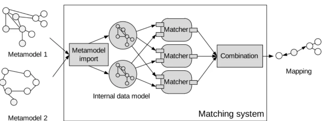
Figure 2.3: Architecture and process of a generic matching system
Definition 2. (Match)The match operator is a function operating on two in-put metamodelsM1andM2. The function’s output is a set of mappings between
the elements ofM1 andM2. Each mapping specifies that a set of elements of
M1 corresponds (matches) to a set of elements inM2. The semantics of a
cor-respondence can be described by an expression attached to the mapping. The match operator is realized by a matching system as described in the following.
2.1.2.1 Architecture of a matching system
A generic representation of a parallel matching system (e. g. [23, 24, 151]) and its components is depicted in Figure 2.3. On the left hand side two input metamodels are given, then they are processed by the matching system (match operator) and an output mapping is created. The matching system
is separated into components as follows:
1. Metamodel import – transforms a metamodel into the matching sys-tem’s internal data model
2. Matcher – calculates a similarity value between all pairs of elements 3. Combination – combines the matcher results to create an output
map-ping
1. Metamodel import The import component transforms a given meta-model into a matching system’s internal meta-model. Thereby, some systems apply pre-processing steps, e. g. [64, 95]. That means they exploit properties of the input metamodels to adjust the subsequent matching process. For instance, the weights of name-based techniques are adjusted if major differences in the element names of the two metamodels are detected.
2. Matcher A matcher calculates a semantic correspondence (match) be-tween two elements. Unfortunately, it has been noted in several publications e.g. [126, 25], that there is no precise mathematical way of denoting a cor-rect match between two elements. This is due to the fact that metamodels (as well as schemas and ontologies) contain insufficient information to pre-cisely define the semantics of elements. Therefore, implementations of the match operator have to rely on heuristics approximating the notion of a correct mapping. A match is realized by a matching technique, which incor-perates information such as labels, structure, types, external resources etc. We define a matching technique as follows:
Definition 3. (Matching Technique)A matching technique is a function map-ping input metamodel elements on a value between 0 and 1;fm:E×E →RN
withes×et7→ [0,1]. This value represents the confidence defined by the
func-tion.
An implementation of a matching technique is a matcher and therefore defined as:
Definition 4. (Matcher)A matcher is an implementation of a matching tech-nique.
Figure 2.2 presents an abstract representation of a matcher. It depicts two given input metamodel elements (along with their corresponding con-text) which are processed by a matcher. Thereby, a matcher makes use of a particular matching technique to derive a similarity. In the subsequent Sec-tion 2.1.2.2 we present a classificaSec-tion and details on matching techniques.
3. Combination The combination component aggregates the results of all matchers and finally selects the output matches as mappings. Thereby, the most common way is to employ different strategies to achieve the aggre-gation of the matcher results [8, 25, 124, 151]. Common strategies are to average the separate results or to follow a weighted approach. Further ex-amples are the minimum, maximum or similarity flooding [107] strategies. The aggregation can be followed by a selection which, for instance, applies a threshold for the similarity value of matches to be considered for the output mapping.
Types of matching systems The matching system depicted in Figure 2.3 implies a parallel execution of matchers which is not obligatory. Indeed, there are three types of matching systems, namely:
• Parallel matching systems, • Sequential matching systems,
• Hybrid matching systems.
Parallel matching systems, e. g. [25], apply each matcher independently on the input metamodels. The matchers are executed in parallel and their result is aggregated. This approach is also followed by MatchBox [151] our proposed system for metamodel matching. In contrast, a sequential matching system, e. g. [37, 38], applies matchers one after another, i. e. a matcher’s result serves as input for the following. This allows for an incre-mental refinement of matching results but may worsen an existing error. Finally, hybrid systems are also possible, for instance [64] use fix-point cal-culations by incrementally executing parallel matchers to use their results as input, again using the same matchers.
Hybrid matching systems have been generalized in meta-matching sys-tems [123]. These syssys-tems are actually composition syssys-tems for matchers. They allow a user to specify the matcher interaction and combination to be applied. Matchers are combined via operators that have an order. This allows, for instance, for an intersection or union of matcher results, thus of matching techniques. In the following section we will classify and detail these matching techniques.
2.1.2.2 Matching techniques
Several matching techniques have been proposed during the last decades originating from the areas of database schema matching, ontology matching, and metamodel matching. For a common understanding of these matching techniques and the self-containment of this thesis we provide an overview of them. The most popular classification of matching techniques has been proposed by Rahm and Bernstein in 2001 [126]. It has been refined and adopted by Shvaiko in 2007 [33] presenting a more complete and up-to-date view on matching techniques. We decided to adopt the classifications of Rahm and Shvaiko in one as outlined in [147]. The combined classification has been developed with respect to the information used for matching, e. g. names (labels) or relations.
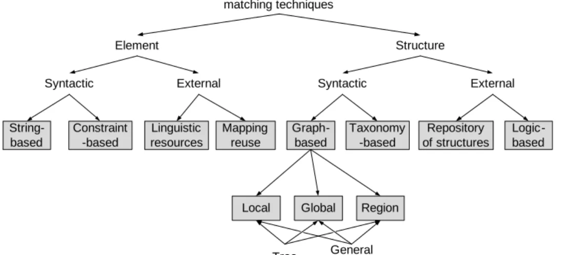
Our classification of matching techniques is given in Figure 2.4. We call the classification adopted because we removed the class of matching tech-niques relying on upper level formal ontologies since it is actually a special form of reuse. We also removed the class of language-based techniques be-cause it actually defines a specialisation of the existing class of string-based techniques. Furthermore, we refined the class of graph-based techniques thus extending the classification.
As can be seen, there are two types of classes: element level and structure-level matching. The types differentiate between techniques operating on elements and their properties and techniques using relations between the elements and thus the structure. Both classes are described in detail in the
String-based Constraint -based Linguistic resources Graph-based Repository of structures Mapping reuse Taxonomy -based Logic-based
Local Global Region
Syntactic External Element Structure Syntactic External Metamodel-based matching techniques Tree General graph
Figure 2.4: Classification of matching techniques
two following sections. Thereby, every technique class will be refined and examples for corresponding matching systems are given.
2.1.2.3 Element-level techniques
Element-level matching techniques make use of information available as properties of elements. In the context of metamodels and our algebraic def-inition, an element is an individual, thus a class, an attribute, a package, an operation, or an enumeration. An element’s label is used for matching. This covers labels such as names, documentation or data types.
String-based String-based techniques cover similarity calculation using string information. Relevant string information includes an element’s name but it also includes metadata such as documentation, annotation, etc. The techniques can be divided into the following three classes:
• Prefix-based calculation uses a common prefix as a base for a heuristics to derive a similarity value.
• Suffix-based calculation is similar to prefix-based calculation but uses a suffix instead.
• Edit-distance-based calculation aims at calculating the number of edit operations necessary to transform one string into another. The more information needed, the less similar two given names are. The most popular approach is the Levenshtein-distance [153].
• N-gram calculation targets the linguistic similarity of model elements. The element labels are split into n-character sized tokens (n-grams). For each token a similarity based on n-grams is computed, which is then the total count of equal character sequences of size n and com-pared to the overall number of n-grams. The resulting ratio is the string similarity.
String-based matching techniques are used by several matching systems in the form of a name matcher [24, 37, 38, 98, 107, 151] or derivations thereof.
Constraint-based Constraint-based matching techniques use information of elements which define a certain constraint on an element. Constraints include data types, keys, or cardinalities. Constraint-based techniques follow the rational that two elements having similar constraints should be similar. Two main classes can be separated:
• Data types are used to derive a similarity of elements based on the data type’s similarity. For simple types such as integer or float a static type conversion table can be used. For complex types such as structures etc. more advanced techniques have to be applied.
• Multiplicity can be used to derive similarity. For instance, similar inter-vals of data types indicate a certain similarity.
Linguistic resources Linguistic resources are used by matching techniques relying on external sources. These external sources can be dictionaries, a common knowledge thesaurus or a domain-specific dictionary. An example for a domain-specific dictionary is a code list, encoding terms in a code as used by SAP [29]. Another popular example is WordNet [39] a publicly available dictionary used for matching.
Mapping reuse Mapping reuse techniques take advantage of mappings already calculated. A prerequisite is a storage for mappings which contains all mappings and the corresponding metamodels in order to reuse these mappings. The most simple approach is using transitivity as an indicator for similarity, i. e. if an elementAmaps onto an elementB, andBmaps onto an elementC, then one may conclude thatAmaps ontoC. Another approach is to use existing matching techniques to derive a similarity between elements to be mapped and already mapped ones, to reuse the knowledge of their mappings.
An example for mapping reuse is COMA [24], which uses fragments that are, as a matter of fact, precisely complex types to derive mappings for the elements [23] referencing those fragments.
(a) Global (b) Local (c) Region
Figure 2.5: Example graph for global, local, and region-based matching con-text; grey highlights the elements used for matching
2.1.2.4 Structure-level techniques
Structure-level based matching techniques follow the rationale ”structure matters”, which is grounded in the theory of meaning [35]. Thereby, it is noted that relations between elements and their position are similar for sim-ilar elements. This structure as encoded in relations, e. g. containment or inheritance, can be used to match different elements. An important aspect of relation-ship matching techniques is the kind of graph they operate on: in the context of matching, two classes are of interest, a general graph and a tree. The following matching techniques can be applied on both. How-ever, a general graph contains more information whereas a tree allows for optimized algorithms reducing complexity especially in terms of runtime.
We distinguish four classes of structure-level matching techniques as de-picted in Fig. 2.5 2: global based, local based, region graph-based, and taxonomy-based matching.
(a) Global graph-based Global graph-based matching uses a complete graph in contrast to local graph-based matching, which only investigates relative elements, e. g. parent elements. Global graph-based matching tech-niques are either exact or inexact.
Exact algorithms describe a mapping from a vertex (element) onto an-other vertex as well as a mapping for edges. Subgraph isomorphism algo-rithms are exact algoalgo-rithms. In contrast, inexact algoalgo-rithms allow for an error-tolerant approach since vertices can be removed or relabelled.
• Exact algorithms, e. g. subgraph isomorphism algorithms, calculate a mapping between two metamodel graphs. The result of an exact algo-rithm is a mapping for each element and relation of one metamodel onto an element or relation of the other metamodel, if and only if they have the same type.
2A circle represents an element where an edge represents a relation, as defined in the convention of Sect. 2.2.2.
• Inexact algorithms such as the graph edit distance or maximum mon subgraph algorithms apply a sequence of edit operations, com-posed of: add, remove, and relabel (rename). A sequence of such op-erations defines a mapping from one graph onto another, thus calcu-lating the maximal common subgraph along with the operations nec-essary.
Global graph-based techniques have not been investigated in depth so far. However, there are selected related results, e. g. a tree-based edit dis-tance approach by Zhang et. al [159], a simplified maximum common sub-graph by Le and Kuntz [92], and an edit distance approach using expecta-tion maximizaexpecta-tion by Doshi and Thomas [27].
(b) Local graph-based Local graph-based matching techniques make use of the context of an element, i. e. the relation of this element to its neigh-bours in a metamodel’s graph. Traditional local graph-based matching tech-niques operate on a tree. Therefore, they use the children, leaf, sibling, and parent relationship, relative to a given element. An extension of these tech-niques is to generalize a graph’s spanning tree and use the neighbours in the graph for matching. Examples for local graph-based techniques are the children, leaf, siblings, and parent matchers in [24, 151]. For a description of those see Sect. 7.2 in our evaluation.
(c) Region graph-based Region graph-based techniques make use of re-gions within a graph, i. e. subgraphs of the complete graph. These subgraphs are studied regarding occurences in the two metamodel graphs and regard-ing the subgraphs’ frequency, i. e. how often they occur in the complete graph. This frequency can be used to derive a similarity between the sub-graphs’ elements. For instance, subgraphs sharing a high frequency are more similar. In contrast to local techniques, the context of region techniques is not restricted to a specific kind of relationship since a frequency is de-termined. An example of region graph-based techniques is the graph min-ing matcher in Section 5.2 in Chapter 5 or the filtered context matcher of COMA++ [25].
Taxonomy-based Taxonomy-based matching techniques operate on the special taxonomy graph in contrast to the general relationship graph. The techniques used for taxonomies are specialized in making use of the tree structure, for instance name path matching and aggregation via super or subconcept rules (parent-child relations).
Repository of structures The approach of a repository of structures is sim-ilar to mapping reuse. A repository contains the mappings, corresponding
metamodels, and coefficients denoting similarities between the metamod-els. The storage of similarities allows for a faster retrieval of mappings for a given metamodel. The coefficients are metrics such as structure name, root name, maximal path length, etc. These numbers act as an index for a set of metamodels, which allows for an efficient retrieval.
Logic-based Logic-based matching techniques make use of additional con-straints defined on metamodels. This covers conditions defined over the metamodels as well as conditions applied to the metamodels. The matching is based on constraints in a logic language, or performed via post processing by adding reasoned mappings. For instance, consider a mapping between attributes, then a mapping between the containing classes has to exist, be-cause attributes need a containing element. Adding this mapping is an ex-ample of logic-based matching.
2.2
Graph Theory
In this section we introduce basic terms such as graphs and labelled graph. The basic terms are followed by a discussion of metamodel graph represen-tations. Subsequently, we define special graph properties which are useful for matching and partitioning and provide the foundations of the fields of graph matching, graph mining, and graph partitioning.
2.2.1 Definitions
Graphs are structures originating from the field of mathematics. They are a collection of vertices and edges, where the edges connect the vertices, thus establishing a pair-wise relation. The first to be known studying graph the-ory is Leonhard Euler in 1736 in his work on the ”Seven Bridge of K¨ onigs-berg” Problem [31]. This work has been refined further and is applied in many areas of today’s computer science, e. g. in path finding problems, lay-outing, search computing, query optimization, etc. A graph is defined as follows:
Definition 5. (Graph)A graphGconsists of two setsV andE,G = (V, E).
V is the set of vertices andE ⊆V ×V is the set of edges.
A graph is called undirected, iff the edge set if symmetric, i. e. withe1 =
(v1, v2) also e2 = (v2, v1) is in E. Otherwise, the vertex pairs defining an
edge are ordered and the graph is called directed.
A graph is finite if the set of vertices is finite. A graph comprising an infinite set of vertices is infinite. Figure 2.6 (a) depicts an example for a graph, showing the vertices (circles) being connected by edges (lines). An
(a) Graph (b) Directed graph E A G C F B D (c) Directed labelled graph
Figure 2.6: Example for a graph, a direct graph, and a directed labelled graph
example of a directed graph is given in the same Fig. 2.6 (b) adding to each edge a direction indicated by an arrow.
Definition 6. (Number of edges/vertices)The number of verticesnis defined asn=|V|. The number of edgesmis defined asm=|E|.
In addition, each vertex and edge of a graph may have a label. A label may represent a colour, type, weight or name of a vertex or edge.
Definition 7. (Labelled Graph)A labelled graphG, is defined as a graph and two labelling functions:fe : E → Le and fv : V → Lv that map edges and
vertices on edge lables and vertex labels, respectively.
Labelled graphs are also called attributed graphs. Whenever referring to a graph in this work we refer to a labelled, undirected, finite graph. An example for a directed labelled graph is presented in Fig. 2.6 (c). Each vertex has an assigned label, in our example a name.
2.2.2 Metamodel representation
Ehrig et al. show in their work [30] that metamodels are equivalent to la-belled, directed, finite graphs (attributed typed graphs extended by inheri-tance). That means for each metamodel a graph exists which has the same expressiveness and allows for the same transformations (graph operations). Even though we could treat metamodels as graphs per se, we base our ob-servations on a metamodel’s mapping on a graph to explicitly discuss the representations of relations, because we want to use the structure for match-ing. The first step towards a metamodel graph mapping is to separate vertex and edge mappings, where:
• A vertex mapping specifies which elements of a metamodel are repre-sented as vertices of the metamodel’s graph,
• An edge mapping defines which metamodel elements relate these ver-tices.
P A a op op() a A A a A P Metamodel Graph
Figure 2.7: Package, class, attribute, and operation mapping onto a vertex
These mappings are based on the graphical representation of a meta-model as defined in [120] or similar in the Unified Modeling Language (UML) [121].
2.2.2.1 Graph-based representation
Vertex mapping The elements which are mapped onto vertices are: pack-age, class, attribute, enumeration, operation, and data type. In the meta-model’s graphical representation they are represented as boxes or parts of boxes.
Figure 2.7 depicts the correspondence between the elements package, class, attribute, and operation and corresponding vertices. In the context of a labelled graph each vertex is labelled according to an element’s name. An additional labelling is the type information, which can also be represented in a graph.
Edge mapping Edges of a graph express relations between vertices. Con-sequently, in a mapping between metamodels and graphs, edges may rep-resent relationships such as inheritance, reference, and containment. These relations are also represented as edges within a metamodel’s graph. The mappings of these relations can be defined as follows:
1. Inheritance can be represented explicitly by edges representing the inheritance relation or implicitly via copying all inherited members in the corresponding subclasses.
2. References and containment can be mapped onto separated edge types. It is important to realize that the mapping between a metamodel and a graph is not unique due to different representations of inheritance relations. For example, Fig. 2.8 depicts an example metamodel and three different graph representations. The metamodel captures common scenarios, where four classes A, B, C, and D are connected by references or containments. A is related to B via bInA, B is related to D via dInB, C is contained in A via the relation cInA, and D is contained in C by dInC. Furthermore, A and D are related by an inheritance, i e. D is a subclass of A.
A B C D bInA cInA dInC dInB Metamodel P P A D
(a) Inheritance graph (b) Reference graph (c) Complete graph P A D B C P A D B C B C
Figure 2.8: Inheritance-, reference-based, and complete graph representa-tion of a metamodel
The first graph (a) is the inheritance-based graph, where only inheri-tance relations are represented as edges. According to the vertex mapping the package P and the classes A, B, C, and D are mapped onto vertices. Ver-tices A and B are connected by a dotted line representing the inheritance. Furthermore, all vertices are connected with the package vertex to guaran-tee the reachability of all vertices, thus there is an edge for each vertex to P.
The reference-based representation (b) is similar to (a), but represents the implicit containment of a package and its classes by edges. Further, A is connected to all vertices B, C, and D, and B and C are connected to D. Finally, the complete graph (c) is a combination of both representations: reference-and inheritance-based.
2.2.2.2 Tree-based representation
Matching techniques such as a parent, children, or leaf matcher3 operate on a tree, because this representation allows for efficient processing of the matcher logic. A tree is a special class of a graph, where each vertex takes part in a parent-child relationship and the graph has a special root vertex. Formally, we define a tree as:
Definition 8. (Tree)A graphGis called a tree, if it has no simple cycle and |V|=|E| −1.
A simple cycle is a traversal of vertices where each vertex is traversed once. The number of edges relates to the number of vertices, because every vertex has at most one parent.
A metamodel does only define one trivial explicit tree. In a metamodel all elements are contained in a package and each package may contain sub-packages. This containment forms an explicit tree consisting of a package as
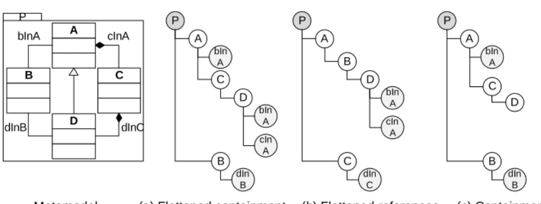
A B C D bInA cInA dInC dInB Metamodel P bIn A cIn A C P B A D
(a) Flattened containment (b) Flattened references (c) Containment
bIn A dIn B cIn A B P C A D bIn A dIn C bIn A C P B A D dIn B
Figure 2.9: Flattened containment, flattened references, and containment tree representations of a metamodel
the root vertex and the contained elements as its children. The leaves of the tree are the attributes of the classes.
However, there are also containment relationships defined via references between classes (marked as containment relations). These relations are also part of the overall containment and should be considered in a tree as well. All of the containment references may form a graph, thus one needs to de-fine a proper tree. In the following the tree definition of a metamodels graph is discussed. Please note that the vertex mapping is analogous to the map-ping on a graph.
Edge mapping The problem consists of a mapping from a graph onto a tree. Several approaches to this problem can be found in literature. The closest one in mapping a meta-model onto a tree is the Minimal Spanning Tree (MST) of a metamodel. A MST is a subgraph of a graph connecting all vertices, thereby forming a tree with the sum of the costs of all edges being minimal. An established algorithm in order to determine the MST of a graph is Kruskal’s algorithm [84].
The mapping onto a tree structure starts with a package and the ele-ments contained. In order to compute the MST first all references and all containment references are handled as edges of a graph. An example of a metamodel mapping is depicted in Fig. 2.9, with three possible MSTs based on the three types of relations.
In Fig. 2.9 (a) the resulting tree is formed by the flattened containment hierarchy, therefore C is contained in A, and D in C, whereas B follows the containment in the package P. The flattened reference import is depicted in Fig. 2.9 (b) having the path A, B, D, because the algorithm takes the left side path first (assuming these elements have been created first). Since we are calculating the MST, no element will have multiple occurrences in the resulting tree.
Besides the problem of defining a proper tree structure, inheritance has to be dealt with. A common approach ignores the semantics of inheritance and discards this information. Alternatively, a metamodel can be flattened, i. e. copying all attributes and relations of a super class into its subclasses. This approach preserves the information defined by inheritance, but loses the connection between super and subclasses. In Fig. 2.9 (a) and (b) a flat-tened import is shown based on the reference and containment hierarchy, whereas (c) shows a non-flattened import, because D does not contain the references inherited from A.
2.2.3 Graph properties
In this section we introduce the graph properties reducibility and planarity. Reducibility is used by our redundancy matcher and planarity in our pla-nar graph-based edit distance matcher as well as in the plapla-nar graph-based partitioning.
2.2.3.1 Reducibility
Reducibility describes the behaviour of a graph under edge contraction. Edge contraction defines the merging of vertices and their edges. If under edge contraction the graph can be contracted into a single vertex, the graph is called reducible. Formally, edge contraction is defined as:
Definition 9. (Edge contraction)Let the graphG= (V, E)contain an edge
e= (u, v)withu6=v. Letf be a function which maps every vertex inV\{u, v} to itself, and{u, v}to a new vertexw.
• The contraction oferesults in a new graph G′ = (V′, E′), whereV′ = (V \ {u, v})∪w,E′ =E\ {e}, and
• For every x ∈ V,x′ = f(x) ∈ V′ is incident to an edgee′ ∈ E′ if and only if the corresponding edgee∈Eis incident to xinG.
The foundation of reducibility are graph minors, which are based on the principle of edge contraction. A minor of a graph is defined as follows:
Definition 10. (Graph minor)An undirected graph H is called a minor of the graph G if H is isomorphic to a graph obtained by zero or more edge contractions on a subgraph ofG.
A minorH ofGthus results from any sequence of edge contraction op-erations on a graphH that lead to a subgraph ofG. The edge contraction is applied on a particular edge by removing it and merging it with its incident vertices. This operation can be applied on a set of edges in any order.
Figure 2.10 shows a minor of a graph along with the edge contraction necessary. The graph in (b) is a minor of the graph in (a), because a sequence
(b) Graph H, Minor of G (a) Graph G a b c (c) Edge contraction
Figure 2.10: Example of a graph, a minor of this graph, and the correspond-ing edge contraction
of edge contraction operations can be defined to form a subgraph. These operations are shown in Fig. 2.10 (c), where three vertices are labelled to explain the operations. First, the edge connecting the vertices a and c is removed and both vertices are merged. The result is a multi-edge between
aand b. Second, one edge of the multi-edge is removed and both vertices are merged. The remaining multi-edge becomes a self-edge ofa. Finally, the self-edge is deleted. The resulting graphHis a minor ofG.
This sequence of edge contraction has also been used in the area of compilers [2]. In this field the analysis of control flow graphs requests for graph (tree) operations such as edge contraction, too. Thereby, use is made of two special transformations,T1andT2. Applying them on a graph in any order defines the reducibility of a graph:
Definition 11. Reducibility LetG = (V, E) be a directed graph where the following transformations are defined:
• T1: Remove a self-edge(v, v)in G.
• T2: If(v, w)is the only edge enteringwandw6=v deletew. Replace all edges(w, x)by a new edge(v, x)and additionally all edges(x, w)by an edge(x, v).
A graph is called reducible, if and only if it can be transformed to a single vertex by applying the two transformations T1 and T2. Otherwise the graph is called irreducible.
2.2.3.2 Planarity
The planarity property of a graph defines when to call a graph planar. It has not been considered for metamodel matching so far. However, planarity al-lows for interesting applications, since graph algorithms requiring planarity can reduce some NP-complete problems to a polynomial, mostly quadratic,
(a) Graph (b) Planar embedding (c) Non planar K5
Figure 2.11: Example of a graph, its planar embedding, and non-planar ex-tension
Non-planar K5 Non-planar K3,3
Figure 2.12: The non-planar graphsK5 andK3,3
runtime when applied on planar graphs. For instance, identifying graph sim-ilarity by subgraph isomorphism calculation on general graphs is known to be NP-complete. If the input graphs are restricted to be planar, the problem can be solved in almost quadratic time. We make use of this property for our planar graph edit distance matcher (Chap. 5) and our planar partitioning (Chap. 6).
An illustrative description of planarity is: A graph is planar, if such draw-ing exists, that none of the graph edges intersect. That means, a graph is planar if it can be embedded into a plane without intersecting edges. This process creates a planar embedding. Figure 2.11 depicts an example for a graph (a) and the corresponding planar embedding (b). As can be seen the example graph is planar. However, if the graph is extended as shown by the dashed line in (c), the graph becomes non-planar, because there is no drawing without intersecting edges.
The graph including the dashed line in Fig. 2.11 (c) is a special graph calledK5, which is one of the two basic non-planar graphs. The other basic
graph is calledK3,3 and consists of six vertices, which are arranged in two
lines of three vertices each with edges between all opposing vertices. Figure 2.12 depicts both graphs.
General graphs
Planar graphs
Trees
Figure 2.13: Subset relation between general graphs, planar graphs, and trees
These graphs are essential for the formal definition of planar graphs, which has been done 1930 in Kuratowski’s theorem [90]. He states:
Theorem 1. A finite graph is planar if and only if it does not contain a sub-graph that is a subdivision ofK5 (the complete graph on five vertices) orK3,3
(complete bipartite graph on six vertices, three of which connect to each of the other three).
Thereby, a subdivision is the result of a vertex insertion in an edge. That means, an edge is split into two edges via a new vertex, still the two new edges connect the original vertices via the new vertex. Instead of using sub-divisions their counterpart, minors, can be used for defining planarity. In 1937 Wagner’s conjecture [152] has been presented and proved in 2004 by Robertson and Seymour [131]. It states:
Theorem 2. (Planar)A finite graph is planar if and only if it does not include
K5orK3,3 as a minor.
According to the definition of a minor, which is a contraction of vertices and their edges, the theorem states, that the graph must not be reducible on either one of the non-planar graphs,K5 andK3,3. Consequently, every tree
is also a planar graph.
The relation between general graphs, planar graphs, and trees is de-picted in Fig. 2.13. The set notation shows the subset relation between the special classes of graphs. Each tree is also a planar graph, where each pla-nar graph (and tree) is naturally a general graph, whereas not every graph is planar or a tree.
The question arises if metamodels are planar and if not, how to make them planar. Both theorems are not suited for a planarity check implemen-tation, but there are algorithms for doing the check with a linear complexity. The most popular one will be described followed by an algorithm to make metamodels planar.
2.2.3.3 Planarity check for metamodels
Metamodels are not planar per se, therefore a planarity check is needed. The planarity check is well-known in graph theory, so we selected in this thesis an established algorithm by Hopfcroft and Tarjan [61], because it has the lowest runtime complexity (O(n)).
The idea of the algorithm is to divide a graph into bi-connected compo-nents (cf. [20], page 11), which are tested for their planarity. Hopfcroft and Tarjan have shown that a planarity of all components results in planarity for the complete graph. The test for each component is done by detecting cy-cles in them. Each cycle is arranged as a path, where non-cycle edges have to be arranged left-hand or right-hand side. Both groups have to contain non-interlacing edges. If for a given edge no group can be found without violating the non-interlacing property, the graph is non-planar. For further details refer to [61].
2.2.3.4 Maximal planar subgraph for metamodels
If a planarity check fails, a metamodel needs to be made planar in order to take advantage of the planarity property. The planarity property can be established by removing vertices or edges. To solve the problem an approach exists where the number of edges is maximal. That means, if an edge that has been previously removed would be re-added, the graph would be non-planar. This algorithm has been proposed by Cai et al. [11] resulting in a complexity ofO(mlogn)(mis the number of edges andnof vertices).
The idea of the algorithm is to recursively compute planar subgraphs of all successors of a particular edge. Afterwards, the subgraphs are combined into one graph by deleting planarity-violating edges. The approach by Cai et al. tests every edge whereas Hopfcroft and Tarjan consider all paths. Fur-thermore, the algorithm by Cai et al.uses a so-called attachment, which is a set of blocks grouping non-interlacing non-cycle edges. The attachments are used to determine the edges to be removed by testing for planarity. Finally, the attachments are recursively merged to construct the maximal planar subgraph. For further details please refer to [11].
The algorithms allow checking any given metamodel for planarity and performing planarisation if necessary. The overall complexity of both opera-tions isO(mlogn)(mis the number of edges andnof vertices).
2.2.4 Graph matching
Graph matching is the similarity calculation of two input graphs. It has first been treated as a mathematical problem but was adopted in several appli-cation domains such as pattern recognition and computer vision, computer-aided design, image processing, graph grammars, graph transformation, and
Graph isomorphism Subgraph isomorphism Exact matching Inexact matching Graph edit distance Maximum common sub-graph Graph matching Probabilistic methods, combinatorial methods
Figure 2.14: Classification of graph matching algorithms adopted from [145]
bio computing [145]. Conceptually, graph matching can be seen as the deci-sion problem whether a graphHcontains a subgraph isomorphic to a graph
G, i. e. if both graphs share similarities. This condition can be relaxed to identifying a subgraph contained in both graphs and even to graphs with a certain distance. Unfortunately, the problem of finding a graph isomorphism for general graphs belongs to NP and is either in NP-complete or P [127]. Therefore, approximations or restrictions on graph properties can be used to cope with the complexity problem. To solve the aforementioned questions so-called graph matching algorithms have been proposed.
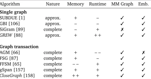
2.2.4.1 Overview of graph matching algorithms
Graph matching algorithms can be divided into two classes: exact and inex-act algorithms. Exinex-act algorithms aim at a subgraph calculation whereas in-exact algorithms are error-tolerant and allow certain distances between the subgraphs. Figure 2.14 depicts a classification provided by [145]. The subse-quent paragraphs deal with the exact, i. e. graph and subgraph isomorphism algorithms, and inexact algorithms, i. e. graph edit distance, maximum com-mon subgraph and combinatorial methods, in detail.
Exact matching Exact matching algorithms aim at calculating for two given input graphs a one-to-one mapping between their vertices and edges. The resulting mapping is a graph isomorphism which is defined as follows:
Definition 12. ((Sub-)Graph Isomorphism). Given a graph Gs = (Vs, Es)
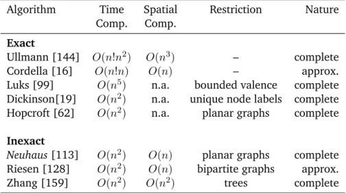
as source andGt= (Vt, Et)as target a graph isomorphism is defined by a
func-tionf :Vs→ Vtsuch that for every edgees = (v, w)alsoet = (f(v), f(w))∈ Et.If|Vs|<|Vt|, then f is called a subgraph isomorphism.
The standard approach on subgraph isomorphism identification is based on backtracking and has been proposed by Ullmann [144] in 1976. Despite being widely referenced the algorithm lacks scalability. That means it is only