Reproducibility in Next-Generation
Sequencing Analysis
Dissertation
zur Erlangung des Grades eines
Doktors der Naturwissenschaften
der Technischen Universit¨at Dortmund an der Fakult¨at f¨ur Informatik
von
Johannes K¨
oster
Dortmund
Dekan: Prof. Dr. Gernot A. Fink 1. Gutachter: Prof. Dr. Sven Rahmann 2. Gutachter: Prof. Dr. Axel Mosig
The analysis of next-generation sequencing (NGS) data is a major topic in bioinfor-matics: short reads obtained from DNA, the molecule encoding the genome of living organisms, are processed to provide insight into biological or medical questions. This thesis provides novel solutions to major topics within the analysis of NGS data, focusing on parallelization, scalability and reproducibility.
The read mapping problem is to find the origin of the short reads within a given reference genome. We contribute the q-group index, a novel data structure for read mapping with particularly small memory footprint. The q-group index comes with massively parallel build and query algorithms targeted towards modern graphics processing units (GPUs). On top, the read mapping software PEANUT is presented, which outperforms state of the art read mappers in speed while maintaining their accuracy.
The variant calling problem is to infer (i.e., call) genetic variants of individuals compared to a reference genome using mapped reads. It is usually solved in a Bayesian way. Often, variant calling is followed by filtering variants of different biological samples against each other. With state of the art solutions, the filtering is decoupled from the calling, leading to difficulties in controlling the false discovery rate. In this work, we show how to integrate the filtering into the calling with an algebraic approach and provide an intuitive solution for controlling the false discovery rate along with solving other challenges of variant calling like scaling with a growing set of biological samples. For this, a hierarchical index data structure for storage of preprocessing results is presented and compression strategies are provided. The developed methods are implemented in the software ALPACA.
Depending on the research question, the analysis of NGS data entails many other steps, typically involving diverse tools, data transformations and aggregation of results. These steps can be orchestrated by workflow management. We present the general purpose workflow system Snakemake, which provides an easy to read domain-specific language for defining and documenting workflows, thereby ensuring reproducibility of analyses. The language is complemented by an execution environment that allows to scale a workflow to available resources, including parallelization across CPU cores or cluster nodes, restricting memory usage or the number of available coprocessors like GPUs. The benefits of using Snakemake are exemplified by combining the presented approaches for read mapping and variant calling to a complete, scalable and reproducible NGS analysis.
The final words I write for this thesis (although presented upfront) are dedicated to those who helped and supported me. Foremost, special thanks go to my advisor Prof. Sven Rahmann. As an employee, I could not imagine a better boss. As a PhD student, I am deeply thankful for enlightening discussions, advice and the many things I learned from him. Furthermore, I want to thank Prof. Axel Mosig for instantly agreeing to become the second examiner of this thesis, as well as Prof. Jens Teubner and Dr. Lars Hildebrand for completing the examination committee.
Thanks go to Dr. Eli Zamir for teaching me about cells and proteins and supporting the development of a feeling for biology. I thank Dr. Alexander Schramm and Prof. Johannes Schulte for almost four years of inspiring cooperation and providing biological motivation for algorithmic work.
Many thanks go to my current and former colleagues Marianna D’Addario, Dr. Daniela Beißer, Dr. Christina Czeschik, Corinna Ernst, Dominik Kopczynski, Prof. Tobias Mar-schall, Dr. Marcel Martin, Christopher Schr¨oder, Henning Timm, Mareike Vogel and Dr. Inken Wohlers for sharing thoughts, providing feedback, having fun in the office and keeping me free of other duties in the decisive last months. Tobias and Marcel should be further thanked for teaching me essential basics during the beginning of my work, transforming me from a student into a PhD student.
I thank the many users of Snakemake for spreading the word about the software and providing feedback. Especially, I thank all early adopters and long-term supporters. For proof reading and trying to understand alien topics, be it computer science, biol-ogy, or even both, special thanks go to Dr. Steven Engler, Stefan Gumprich, Dominik Kopczynski, Nicolas Potysch, Sven Strothoff and Martina Weiss. You provided extraor-dinarily helpful feedback.
I thank my parents and my parents-in-law for all their support and advice. Finally, I thank my wife Christine for her enormous support, love and patience in case of long work days, weeks of absence during conferences and delayed answers while sitting in front of my laptop or writing on the ugly whiteboard in our living room.
Johannes K¨oster
1 Introduction 9
1.1 The genome . . . 10
1.2 Next-generation sequencing . . . 12
1.3 Designing for efficient GPU usage . . . 14
1.3.1 Parallel random access machines . . . 15
1.3.2 Prefix scans . . . 16
2 A massively parallel read mapper 19 2.1 Introduction . . . 19 2.2 Related work . . . 22 2.3 Q-gram index . . . 24 2.4 Q-group index . . . 24 2.4.1 Size . . . 27 2.4.2 Construction . . . 28 2.5 Algorithm . . . 31 2.5.1 Filtration . . . 32 2.5.2 Validation . . . 35 2.5.3 Postprocessing . . . 36 2.6 Results . . . 38
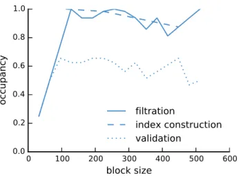
2.6.1 GPU resource usage . . . 38
2.6.2 Sensitivity . . . 39
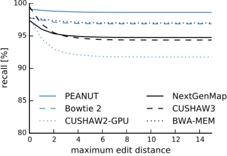
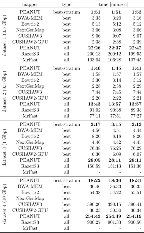
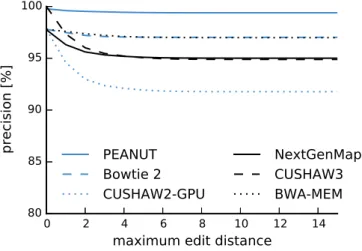
2.6.3 Comparison with other read mappers . . . 40
2.6.4 Profiling algorithm steps . . . 45
2.6.5 Evaluation of mapping qualities . . . 46
2.7 Discussion . . . 47
3 An algebraic variant caller 49 3.1 Introduction . . . 49
3.2 Related work . . . 52
3.3 Bayesian variant calling . . . 56
3.4 Algebraic variant calling . . . 62
3.5 Applications of algebraic variant calling . . . 65
3.6 Algorithm and data structure . . . 67
3.6.1 Sample indexing . . . 68
3.6.2 Index merging . . . 69
3.6.4 Compression . . . 70
3.6.5 Implementation . . . 74
3.7 Results . . . 76
3.7.1 Compression . . . 77
3.7.2 Comparison with other variant callers . . . 79
3.8 Command line interface . . . 85
3.9 Discussion . . . 86
4 A scalable text-based workflow system 89 4.1 Introduction . . . 89
4.2 Related Work . . . 91
4.3 Workflow definition language . . . 92
4.3.1 Defining resource usage . . . 95
4.3.2 Temporary and protected files . . . 96
4.3.3 Additional functionality . . . 96 4.3.4 Python rules . . . 98 4.3.5 Modularization . . . 98 4.3.6 Parsing . . . 99 4.4 Dependency resolution . . . 102 4.5 Job scheduling . . . 105
4.6 Support for distributed computing . . . 109
4.7 Data provenance . . . 109 4.8 An example workflow . . . 111 4.9 Discussion . . . 115 5 Conclusion 117 A Appendix 119 A.1 Software . . . 119
A.2 Contributions to co-authored articles . . . 120
The genome of a living organism encodes its hereditary information. It serves as a blueprint for proteins, which form living cells, carry information and drive chemical reactions. Differences between populations, species, cancer cells and healthy tissue, as well as syndromes or diseases can be reflected and sometimes caused by changes in the genome. This makes the genome an major target of biological and medical research. Today, it is often analyzed with next-generation sequencing, producing gigabytes of data from a single biological sample. Analyzing this data entails creating complex workflows with tens of steps, applying various tools and converting between diverse representations of information. Two steps common to many such analyses areread mapping andvariant calling. This thesis presents novel algorithms and data structures for read mapping and variant calling, and a workflow system that supports the analysis of next-generation sequencing data in a reproducible way.
For read mapping, we present the q-group index, a novel index data structure with a particularly small memory footprint, complemented by parallel algorithms for querying and building the index, targeting graphics processing units (GPUs). On top, we provide the novel read mapper PEANUT. By effectively exploiting parallelization on GPUs, it outperforms other read mappers while maintaining their accuracy.
With the variant caller ALPACA, we present an algebraic approach to variant calling, that is the first to allow intuitive control of the false discovery rate in complex filtering scenarios. ALPACA is designed to parallelize well on both central processing units (CPUs) and GPUs. We explore the use of hierarchical index data structures and their compression, ensuring scalability with the number of considered biological samples. Finally, we present the workflow system Snakemake. While being designed with next-generation sequencing analysis in mind, it provides a general purpose, text-based, easy to read domain-specific language for workflow definition. Snakemake workflows entail implicit parallelization and scale from single-core workstations and multi-core servers to compute clusters without changing the workflow definition. The scheduling of Snake-make can be made aware of arbitrary resources, e.g., restricting the number of available GPU devices. Support for documentation and data provenance further enhance the reproducibility of Snakemake workflows.
The chapters 2 to 4 contain the three major topics of the thesis. Each chapter has its own introduction, providing the foundations needed for that chapter and a separate discus-sion summarizing the findings and outlining future work. Chapter 2 describes the read mapping problem and presents the q-group index data structure in combination with
the read mapper PEANUT as a massively parallel, efficient solution exploiting modern graphics cards. Chapter 3 describes the variant calling problem and shows how to solve it with the variant caller ALPACA in an algebraic approach, while keeping paralleliza-tion and scalability in mind. Chapter 4 introduces the workflow system Snakemake, defining the entailed domain-specific language and the scalable scheduling. The chapter ends with an example workflow which models a complete next-generation sequencing analysis combining the approaches from Chapter 2 and 3. The thesis is closed with the concluding Chapter 5. In the appendix, co-authored articles and the software pub-lished with this thesis are summarized. In the following, we introduce biological and algorithmic foundations that are particularly important in the context of this work.
1.1 The genome
We briefly introduce the necessary biological foundations based on the description of Alberts, Johnson, and Lewis (2008). The genome is encoded by deoxyribonucleic acid (DNA) molecules. DNA is a sequence of smaller units, the nucleotides. A nulceotide consists of a sugar (here deoxyribose), a phosphate group and an organic base. Within DNA, nucleotides with the bases adenin (A), cytosin (C), guanin (G) and thymine (T) occur. The nucleotides are connected via covalent bonds between the sugar of one and the phosphate of the next nucleotide. Hence, a DNA molecule has a direction, starting with a free sugar and ending with a free phosphate. The two ends are called 5’ and 3’. When encoding the genome, DNA molecules occur double stranded, forming a helical structure, called the double helix. In this form, the two DNA strands are connected to each other via hydrogen bonds between their bases: A can bind to T, and C can bind to G. We say that A is complementary to T, and C is complementary to G. One strand is the reverse complement of the other, i.e., the 5’ (first) base of the first strand is complementary to the 3’ (last) base of the second strand, and so on. This maximizes the number of bonds between the two strands. From computer science perspective, a DNA strand can be seen as a string over the alphabet{A,C,G,T}. We interchangeably refer to A,C,G and T as bases, nucleotides or basepairs (referring specifically to their paired form in the double strand).
The storage of genomic DNA within a cell allows to divide species into prokaryotes (e.g., bacteria) and eukaryotes (e.g., mammals). The former consist of a single cell and their hereditary information is carried by a circular double stranded DNA molecule that may exist in multiple copies. In contrast, the DNA of eukaryotes is contained in a membrane surrounded structure, the nucleus, and occurs aschromosomes. A chromosome is a sin-gle, coiled, double stranded DNA molecule. Eukaryotic cells can have multiple copies of each chromosome. The number of copies is calledploidy.Diploid organisms like humans have in general two copies of each chromosome. An exception are the sex chromosomes X and Y: female individuals have two X chromosomes and no Y chromosome, males have an X and a Y chromosome. One copy of each chromosome is inherited from the mother, one from the father.
C T C G A G G A A T C G C A G C G C A T C A A C A C T C G A G G A A T C G C A G C G A A T C A A C A Figure 1.1: Example DNA sequences within two copies of the same chromosome of a
diploid genome. We omit the sequence of the reverse complementary strands. The dashed box depicts a homozygous locus, the dotted box shows a het-erozygous locus. The former has genotypeGG, the latter exhibits the geno-typeCA. Combinations of alleles on the same chromosome depicted by solid lines are two haplotypes that can be observed here (GC andGA).
Each chromosome hosts a set of genes. Genes are segments in the DNA that encode instructions for creating a product. Usually, this product is aprotein. Proteins are chains of amino acids, that execute various functions within the cell, build organelles and signalling channels, and form complexes. They are synthesized from genes in two steps. First, a gene istranscribed into an intermediate copy of itself in the form of ribonucleic acid (RNA) via the RNA polymerase enzyme. RNA is similar to DNA, having a ribose instead of deoxyribose sugar and a uracil (U) nucleotide instead of thymine. Second, the RNA molecule, called messenger RNA (mRNA) is translated into a protein by the ribosome, which itself is a complex of proteins. Each three consecutive nucleotides (called codon) in the mRNA encode for one amino acid. Genes are partitioned intoexons
andintrons. Exons are the coding regions of a gene: during transcription, intronic regions are spliced out, i.e., they do not encode the amino acids that end up in the protein. The set of all exons of a genome is calledexome.
The terms explained in the following are illustrated in Figure 1.1. Depending on the ploidy, each gene can be present in one or more copies of a chromosome. The different copies of a gene are called alleles. In this thesis, following DePristo et al. (2011), we also apply the term allele to individual positions on a chromosome, independently of the genes. In other words, alleles can also be the different bases occurring at the same position in all copies of a chromosome. With locus, we refer to a particular position on all copies of a chromosome. In a diploid organism, except on the sex chromosomes, each locus hosts two alleles. In an individual, the combination of all alleles of the same gene or locus is called genotype. In contrast, the combination of alleles of different loci on the same copy of a chromosome is called haplotype. The genomes of different individuals of the same species are, while being similar, not entirely the same.Mutations
can cause nucleotide-level or even larger changes from one to the next generation (see Chapter 3). Even within a single individual, a locus may exhibit different alleles. We call such loci heterozygous. Loci which host the same allele on all chromosomes are called
homozygous.
Eukaryotic genomes can be huge: e.g., the human genome has about 3.2 billion bases distributed to 24 different chromosomes and 25 thousand genes (Alberts, Johnson, and
Lewis 2008). Hence, the sequencing of genomes and the analysis of the obtained data is particularly challenging.
1.2 Next-generation sequencing
Sequencing of DNA is the determination of the nucleotide sequence of a DNA molecule. For long, the primary method of DNA sequencing was Sanger sequencing, proposed by Sanger, Nicklen, and Coulson (1977). In a huge and costly effort, the Sanger method al-lowed to initially sequence the human genome (Lander et al. 2001). From 2005 to 2008, a new class of sequencing methods emerged, which are commonly referred to as second- or
next-generation sequencing (NGS). Shendure and Ji (2008) identify three steps common to all NGS approaches. First, the DNA subject to sequencing is fragmented randomly, and artificial adapter DNA molecules are attached. The resulting sequences are ampli-fied (i.e., duplicated several times) with a polymerase chain reaction (PCR; see Mullis, Ferre, and Gibbs (1994)) and localized in clusters of duplicate single stranded fragments on some carrier material. Finally, the sequencing of the fragments is performed by cycles of biochemical treatment and imaging based data acquisition. The PCR amplification is necessary to make the signal detectable by the imaging. Together, ncycles yield the sequence of the first n nucleotides of all fragment clusters in parallel. We call these sequencesreads. Read lengths range from 32 to a few hundred, with 100 to 200 being a common size in current studies.
Today, the most popular (Lam et al. 2012) implementation of next-generation sequenc-ing is sold by Illumina1. With this technology, also called SBS (sequencing by synthesis), each cycle works as follows. First, a solution of free nucleotides is flooded over the frag-ment clusters. A DNA polymerase now synthesizes at each originally single stranded fragment another nucleotide of the reverse complementary strand (synthesis). The nu-cleotides are equipped with a fluorescent label, with different colors for A, C, G and T. The label prevents the synthesis of more than one nucleotide per cycle. At the end of each cycle, remaining free nucleotides are washed away (washing), the fluorescent color of each cluster is measured, providing information about the nucleotide attached in that cycle, and the nucleotide labels are removed (label removal), allowing the synthesis of another nucleotide in the next cycle. Figure 1.2 shows an example.
Compared to Sanger sequencing, NGS is less accurate: the observed error rates with Sanger sequencing range from 0.01% to 0.001% (Kircher and Kelso 2010). With Illumina sequencing, error rates of 1% are observed (Ross et al. 2013). In return, NGS yields more reads (hundreds of millions) at low costs.
An important variant of the sequencing protocol is paired-end sequencing. Here, frag-ments are sequenced from both ends. This results in two reads per fragment cluster, which are known to come from the same fragment. Usually, the size of the fragments
fragment G A A T C G C A G C G C A read C T T A G A G T synthesis washing label removal
Figure 1.2: Next-generation sequencing cycle with Illumina SBS. Free labelled nu-cleotides are used to synthesize the next read base. Then, remaining free nucleotides are washed away and the synthesized read base is determined by its label. Finally, labels are removed.
(called insert size) is controlled, such that a certain distance between the read pairs can be expected. Paired-end sequencing has several advantages: e.g., it helps to find the true origin of ambiguously mappable reads (see Chapter 2). It can also be used to detect structural variants (Marschall et al. 2012) or help to infer transcript expressions (Trapnell et al. 2010).
With automated sequencing technologies being in place since about 30 years, the genomes of many species are well known by now. These reference genomes are representative mixtures, assembled from several individuals. Various applications of NGS have been developed that make use of an already known reference genome. Here, the read map-ping problem occurs: for the reads obtained from the biological sample, the origin in the genome is unknown. Theread mapping problem is to determine this origin by find-ing the most likely position of each read within the reference genome (see Chapter 2). When sequencing DNA, comparisons of the differences between reads and the refer-ence genome can be used to detect genomic variants (see Chapter 3). Further, e.g., RNA can be sequenced to quantify the expression of genes and transcripts (RNA-seq; Wang, Gerstein, and Snyder 2009), and binding sites of transcription factors can be determined by combining NGS with antibody-based selection of fragments (ChIP-seq; Park 2009). The sequencing of DNA can also be targeted towards exonic regions (exome sequencing). With only about 1.5% of the 3.2 billion bases of the human genome being exonic (Alberts, Johnson, and Lewis 2008), the capacity of the sequencer can be used to generate a much higher read depth at the expense of loosing intronic and intergenic regions, without increasing or even lowering sequencing costs.
Reads are typically provided in the FASTQ format (Cock et al. 2010). The format pro-vides read bases as a string over the IUPAC alphabet2 which encodes in addition to Σ ={A,C,G,T}classes of uncertain bases with additional letters, e.g., an N represents that the base is entirely unknown, a W represents uncertainty between A and T. Typi-cally, only Ns occur in addition to Σ. Along with each base, a base quality is provided.
The quality is the probability that the base was miscalled by the sequencer, given in the so-called PHRED scale: Letpbe a probability, then the PHRED scaled probability is obtained as
q :=−10 log10p.
With FASTQ, the PHRED-scaled base qualities are stored in single bytes, allowing to encode miscall probabilities from 1.0 to 10−9.3.
In the context of this thesis, the term sample will, if not stated otherwise, usually describe a sample from some biological tissue that has been sequenced by some NGS technology to obtain reads.
1.3 Designing for efficient GPU usage
Chapter 2 and 3 present parallel algorithms targeted towards GPUs. This requires architecture specific considerations, which we elaborate here based on the work of K¨oster and Rahmann (2014). We first describe the GPU architecture and its implications. Then, we define the parallel random access machine (PRAM) that serves as an abstraction for assessing the time complexity of parallel algorithms. Finally, we introduce the prefix scan programming pattern that is used widely in this work.
We use the terminology of NVIDIA3, while the general concepts are also applicable to the hardware of competitors like AMD4. A GPU is partitioned into Streaming Mul-tiprocessors (SMs), each of which has its own on-chip memory, cache and processing cores. By adjusting thethread block size it can be controlled how threads are distributed among the SMs. One thread block is executed on one SM and stays resident until all threads in the block are completed. Once a thread block is finished, another will be scheduled to the SM if any blocks are left. An SM can execute 32 threads in parallel (restricting the thread block size to be a multiple of 32); such a group of threads is called awarp orwavefront. At any time, each of these threads has to execute the same instruction in the code, but may do so on different data; this concept is called sin-gle instruction, multiple threads (SIMT). Hence, conditionals with diverging branches should be avoided, since threads taking an if-branch have to wait for threads taking the corresponding else-branch to finish and vice versa. All SMs may access a slow common global memory (often less than 3 GB) in addition to their fast on-chip cache and mem-ory. While the size of the fast cache is extremely limited, accessing global memory is slow and should be minimized. The memory latency can be reduced by coalescing the access, i.e., letting threads in a warp access contiguous memory addresses, such that the same memory transaction can serve many threads. In addition, an SM can execute a different warp while waiting on a transaction to finish, thereby hiding the latency. For the latter, threads should minimize their register usage such that the number of warps
3
http://www.nvidia.com, visited 11/2014
that can reside on an SM is maximized. Finally, data transfers from the main system memory to the GPU’s global memory are comparatively slow. Hence, it is advisable to minimize them as well.
To implement parallel algorithms for both GPU and CPU, we use OpenCL5. With OpenCL, parallel algorithms are implemented as kernels in OpenCL-C, a dialect of the C language. For given input data, typically in the form of one or more arrays, a kernel is executed with potentially many threads. Each thread executes the kernel code on one or more data points of the input data: e.g., a kernel executing withn threads can replace a loop overn items of an array. The kernel code would be equal to the body of the loop here. OpenCL provides an API for accessing various compute devices (e.g., the CPU or the GPU), managing memory and launching kernels. As all provided software is implemented in the Python programming language6, we use the Python package PyOpenCL (Kl¨ockner et al. 2012) to access OpenCL from within Python.
1.3.1 Parallel random access machines
A parallel random access machine (PRAM) is a theoretical model for analyzing parallel algorithms, defined as a collection of synchronous processors that have random access to a common shared memory (Dehne and Yogaratnam 2010; Reif 1993). The behavior of different processors accessing the same memory unit classifies PRAMs into
1. the EREW (exclusive-read, exclusive-write) PRAM, which allows only one pro-cessor at a time to read from and write to a memory unit,
2. the CREW (concurrent-read, exclusive-write) PRAM, which allows multiple pro-cessors at a time to read from a memory unit and only one to write,
3. the CRCW (concurrent-read, concurrent-write) PRAM, which allows multiple processors at a time to read from and write to a memory unit.
The PRAM abstracts from caching and communication between threads. In principle, a GPU could be seen as an CRCW PRAM, since it has multiple processors that can concurrently write to and read from a common memory. We choose to assess time complexity of the algorithms presented in this work with the PRAM model. Some of the presented algorithms require exclusive access to a memory unit (e.g., an entry within an array) for certain operations like counting, which we implement with OpenCL atomic operations7. Hence, we conservatively decide to assess complexity under the CREW PRAM model.
In practice, there are differences between the PRAM and a GPU (Dehne and Yogarat-nam 2010). First, the processors of a GPU are grouped into SMs, the processors of which
5 https://www.khronos.org/opencl, visited 11/2014 6http://www.python.org, visited 11/2014 7 https://www.khronos.org/registry/cl/sdk/1.2/docs/man/xhtml/atomicFunctions. html, visited 11/2014
can only work in parallel if they execute the same instruction. Second, memory accesses that do not coalesce between the processors can impact the performance. Hence, we complement the PRAM-based theoretical complexity results with discussions of GPU specific optimizations.
1.3.2 Prefix scans
A useful programming pattern that is used extensively in the algorithms presented in this work are parallel prefix scans (see Cormen et al. 2001; Blelloch 1990). A special case of prefix scans is the computation of a cumulative sum, which at first appears to be a serial process. Parallel prefix scans are used to solve these problems in a data parallel way with a minimum amount of branching, thus nicely fitting above considerations for GPU programming. In the following, we first define the prefix scan operation and then discuss its parallel implementation on a PRAM as presented by Blelloch (1990).
Definition 1.1 (Prefix scan). Let A= (a1, a2, . . . , an) be a sequence ofnelements and ⊕be an associative operator. Then, the prefix scan on A with operation ⊕ is given as
(a1, a1⊕a2, . . . , a1⊕a2⊕ · · · ⊕an).
In the following, we refer to this operation as the scan operation. We further call a scan onA0 = (e, a1, a2, . . . , an−1) withebeing the neutral element of⊕, the prescan on
A. While scan and prescan appear to be inherently sequential, they can be efficiently parallelized on a PRAM with ρ processors. In the following, we outline a parallel im-plementation of the prescan (Blelloch 1990). The scan can be obtained from this by removing the leading e and appending the ⊕-sum of an and the last element of the prescan.
The idea is to explore the levels of a binary tree with heightdlog2neover the sequence. The nodes of the binary tree shall represent intermediate results of our computation. Initially, the leaves of the tree are determined by the values of the sequence. We calculate the values of each level iteratively, overwriting previous results in place, i.e., we map the value of thei-th node (from left to right) with heighth at elementak withk= 2hi. On each level, the values of each node are calculated in parallel from those of the previous iteration. To obtain a prescan, we perform three steps (see Figure 1.3):
1. Explore the binary tree bottom-up, and set the value of each vertex to the⊕-sum of its children.
2. Set the root to the neutral element.
3. Explore the binary tree top-down in preorder. For each node with valuev set (a) the value of the right child to the⊕-sum of the value of the left child andv and set (b) the value of the left child tov.
25 11 14 4 7 5 9 3 1 7 0 4 1 6 3 ⊕ = 0 0 11 0 4 11 16 0 3 4 11 11 15 16 22 11⊕ =
Figure 1.3: Example for the parallel implementation of the prescan operation with ⊕ being the addition and neutral element 0. The algorithm first calculates the left tree bottom up and then the right tree top down. The node values of each level are calculated in parallel.
After step one, element k = 2hi of the sequence contains the result of a1⊕ · · · ⊕ak. In step three each node shall be set to the sum of all leaves preceding it according to the preorder traversal. Since the root is preceded by no leaf, we set the root node to 0 in step two. After step two, the sum of the leaves preceding the right child is always equal to the sum of the left child after step one and the value of the parent. Hence, substep (a) of the third step sets the right child to that value. The left child has the same preceding leaves as the parent, therefore the value of the parent can be copied in substep (b). A detailed proof for this concept is presented by Blelloch (1990).
Usually, there will be more values in the sequence than processors on the PRAM, i.e., n > ρ. Then, the sequence can be divided into partitions of size dn
ρe. For each partition, the ⊕-sum and the prescan can be calculated sequentially by one of the PRAM processors and used as leaves of the tree. The prescan of the⊕-sums can then be used as an offset for a prescan over each partition. This leads to a time complexity of O n ρ + log2ρ (1.1) composed of the time for calculating the partition sums and calculating theh= log2ρ levels of the tree in parallel on an EREW PRAM (Blelloch 1990).
An example application of a prefix scan is to calculate a predicated copy of a sequence: from a sequenceA= (a1, a2, . . . , an) and a predicate f :A→ {0,1}assigning a boolean value to each element of A we want to generate the sequence A0 of exactly those el-ements ak ∈ A where f(ak) = 1. To achieve this, we calculate the prescan over the sequence (f(a1), f(a2), . . . , f(an)). This generates a sequenceB where thek-th element denotes the target address of elementak withf(ak) = 1 in the predicated copyA0: e.g., consider a sequenceA= (1,7,3,4,5) with predicatef(ak) =1ak>3 being the indicator
(0,1,0,1,1), resulting in the sequenceB= (0,0,1,1,2). By copying elementsa2,a4 and
a5 to the corresponding addresses specified in B we obtainA0= (7,4,5).
PyOpenCL (see Section 1.3) provides a flexible mechanism of defining prefix scans using templates. Further, it implements various primitives via prefix scans, e.g., cumulative sums and predicated copies.
Next-generation sequencing produces millions of small reads that represent the DNA sequence of a biological sample (or specific parts thereof; see Section 1.2). The read lengths range, depending on the technology and biological question, from tens to sev-eral hundreds of bases. Today, read lengths of 100 – 200 are common. Typically, a genomic region is covered by more than one read but the information about the orig-inating position of each read in the genome is lost during the sequencing process. For many species, a reference genome, representing a consensus among several individuals is already known (see Section 1.1). The read mapping problem is to find the origin of each read in the reference genome. Here, we present a novel data structure that helps to solve the read mapping problem efficiently on GPUs. On top of this, we introduce a new read mapping algorithm.
2.1 Introduction
In the following, we denote the set of strings over an alphabet Σ as Σ∗. Depending on the context, we call a string also word or text. We denote withs[i] thei-th character (or letter) of a strings∈Σ∗. Further,s[i, i+k] denotes the substring of length kbeginning at positioni. The term|s|refers to the size of strings. The empty string is denoted as εand ◦ is the string concatenation. We denote the set ofk-combinations over a setM asMk.
The reference genome usually consists of multiple sequences (i.e., chromosomes). We denote these as the reference sequences. We interpret the reference sequences and any read as strings over the alphabet Σ = {A,C,G,T}. Since a read can come from ei-ther strand of the chromosome (see Section 1.1) we also have to consider the reverse complement of each reference sequence.
An exact occurrence of the read in a reference sequence or its reverse complement is the most likely origin of a read. Therefore, at first sight, the read mapping problem can be approached by finding all occurrences of a patternP in a text T, namely applying classicalpattern matching (see Cormen et al. 2001), withP being a read, andT being a reference sequence or its reverse complement. Pattern matching searches for all positions iin a text T such that P is a substring of T beginning at positioni.
In practice, many reads will not match exactly to their origin because of two reasons. First, the sequenced sample will have local differences to the reference due to the natural
genetic variation (see Section 1.1). Second, the sequencing itself can introduce technical errors and artifacts. Within reads, these differences manifest assubstitutions,insertions
anddeletions of bases compared to the reference sequence. Therefore, the matching has to be approximate (or error tolerant), leading to alignments (see Gusfield 1997) of the reads against the reference sequences:
Definition 2.1 (Alignment). Let s, t∈Σ∗ be two strings over an alphabet Σ. A global
alignment A of s and t is a string over the alphabet Σ0 = (Σ∪ {−})2 \ {(−,−)} with
π1(A) = s and π2(A) = t. Here, π1 and π2 are homomorphisms with π1((a, b)) := a,
π1((−, b)) =ε,π2((a, b)) :=b,π2((a,−)) =εandπi(B◦C) =πi(B)◦πi(C)fora, b∈Σ,
B, C ∈Σ0∗ and i∈ {1,2}.
We call the global alignment of substrings of s and t a local alignment, and the global alignment of sagainst a substring of t a semi-global alignment.
When printing the pairs of the alignment alphabet as columns, one (but not necessarily the best) global alignment between the stringsEAT and PEANUTis:
-EA--T PEANUT
The quality of an alignment can be assessed using a distance measure dthat typically quantifies the amount of edit operations needed to turn one string into the other. In the following, we will sometimes call edit operations errors and use the term error rate as a synonym for a distance measure. For the read mapping problem, it suffices to con-sider substitutions, insertions and deletions as edit operations. Theedit orLevenshtein distance (Levenshtein 1966) weights each operation equally, and can be written as
d(sa, tb) = min d(s, t) +1a6=b, d(s, tb) + 1, d(sa, t) + 1 (2.1)
withd(s, ) =|s|,d(, t) =|t|,s, t∈Σ∗ anda, b∈Σ (Navarro and Raffinot 2008). Here,
1a6=b is the indicator function evaluating to 1 if a6=b and 0 otherwise. Further,sa and tbare the stringssandtextended by the lettersaandb, respectively. In the recurrence, the first case handles substitution and match, followed by deletion from and insertion into s. Alternatively, the quality can be calculated via an alignment score. Alignment scores often weight matching characters with 1, penalize substitutions with−1 and use affine costs for insertions and deletions (also calledaffine gap costs), i.e., opening a gap has a higher cost than extending it. Edit distances or alignment scores and (optionally) the concrete alignment can be calculated by variants of the Smith-Waterman algorithm (Smith and Waterman 1981), which makes use of the score (or edit) matrix E. For stringss and t, the matrix contains one row for each letter a∈ sand one column for each letter b ∈ t. The value Eij is the maximal score (or minimal distance) between a prefix of s of length i and a prefix of t of length j. Interpreted as a graph with a node for each matrix entry and directed edges from (i, j) to (i+ 1, j+ 1),(i, j+ 1) and
(i+ 1, j), a path in E represents a local alignment between s and t. A path from the top to the bottom row represents a semi-global alignment whereas a path from the top left to the bottom right represents a global alignment. The variant that finds the latter path is also called Needleman-Wunsch algorithm (Needleman and Wunsch 1970). The Smith-Waterman Algorithm explores the score matrix with dynamic programming in time complexity O(|s| · |t|) to find the best alignment score. Backtracking can be used to reconstruct a concrete alignment for the best score.
Now, the read mapping problem can be solved by finding the best semi-global alignment (according to some distance measure) of a read against the reference sequences and their reverse complements. Sometimes, the reads are expected to exhibit larger differences to the reference than local substitutions or small insertions or deletions. For example, they may contain technical adapters at one end (see Section 1.2), or a read may span a structural variant (e.g., a fusion of two chromosomes) that occurs in the sequenced sample. When this can be expected, it is advisable to look for local alignments instead of semi-global alignments, allowing to omit larger parts of a read without penalizing them in the distance measure.
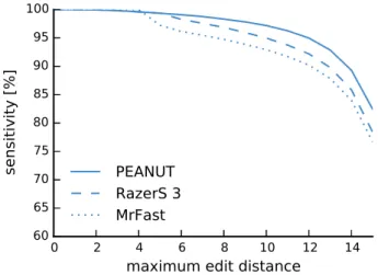
The sizes of genomes (approximately 3.2 billion basepairs for human, 2.7 billion base-pairs for mice; see Section 1.1) and the hundreds of millions of reads produced by a single modern next-generation sequencing experiment, render the application of the Smith-Waterman algorithm for each read against the complete reference prohibitive. Hence, various filtering methods and approximations have been developed. These can be roughly classified into methods based on backward search using the Burrows-Wheeler Transform (BWT; see Section 2.2) and methods based on q-gram indexes (see Sec-tion 2.3). Examples for the former are BWA (Li and Durbin 2009) and Bowtie 2 (Lang-mead and Salzberg 2012), examples for the latter are RazerS 3 (Weese, Holtgrewe, and Reinert 2012) and MrFast (Alkan et al. 2009).
Among the best alignments of a read, it is sometimes not obvious which one represents the true origin of the read. In the following, the candidate origins of a read reported by a read mapper are calledhits. Weese, Holtgrewe, and Reinert (2012) categorize read mapping implementations into best-mappers that try to find the (or any) best hit of a read (e.g., BWA-MEM) and all-mappers that provide a comprehensive enumeration of all possible locations (e.g., RazerS 3 or MrFast) up to a given error threshold. While all-mappers can be much slower (depending on the number of hits), their strategy is beneficial whenever suboptimal hits are of relevance. For example this is the case when the originating genome of the reads is unknown (e.g., when sequencing a mixture of samples). Roberts and Pachter (2013) mention the mapping to alternative transcripts (see Section 1.1) and Alkan et al. (2009) motivate all-mapping with the detection of copy number variations (i.e. duplications of parts of chromosomes). An intermediate strategy is to report all hits of the best stratum, i.e., all hits with the same lowest error level (instead of only the first or a random such hit).
Recently, exploiting the parallelization capabilities of GPUs for read mapping has be-come popular and GPU-based BWT read mappers appeared, e.g., SOAP3 (Liu et al.
2012), SOAP3-dp (Luo et al. 2013) and CUSHAW2-GPU (Liu and Schmidt 2014). Using a q-gram index on a GPU is not a common choice because of its large size. Therefore, to the best of our knowledge, q-gram based mappers so far only use the GPU for cal-culating the alignments and keep the index on the CPU, e.g., NextGenMap (Sedlazeck, Rescheneder, and von Haeseler 2013) and Saruman (Blom et al. 2011).
Here, by introducing the q-group index, a new approach to solving the read mapping problem on the GPU is presented. The q-group index is a variant of the traditional q-gram index, with a smaller memory footprint. We show how the q-group index can be efficiently built and queried on GPUs using parallel algorithms. The q-group index is used in afiltration and validation approach: Exact matches of a given lengthq between each read and each reference sequence are detected quickly and alignments are computed only where such matches are found. The resulting read mapper is called PEANUT (ParallEl AligNment UTility) and available as open source software under the MIT license (see Section A.1).
This chapter is based on previously published work (K¨oster and Rahmann 2014). First, related work is summarized (Section 2.2). Then, the traditional q-gram index is intro-duced (Section 2.3). Next, the novel q-group index (Section 2.4) and the read mapping algorithm of PEANUT (Section 2.5) are defined. The chapter ends with evaluations of the performance and accuracy, comparing PEANUT with other read mappers (Sec-tion 2.6) and a discussion (Sec(Sec-tion 2.7).
2.2 Related work
We describe BWA and RazerS 3 as representatives of BWT and q-gram index based approaches. Additionally, we describe the two GPU based read mappers CUSHAW2 and NextGenMap.
BWA A popular read mapper is BWA, the Burrows-Wheeler-Aligner (Li and Durbin 2009), which simulates an error tolerant search in a suffix array using the BWT. For a textT over an alphabet Σ ended by a sentinel $ that is lexicographically smaller than all other letters in the text, the suffix array S is a permutation of the text positions such thatS[i] is the start position of the i-th suffix according to lexicographical order. The BWT B of the textT is a permutation of T such that the i-th position contains the character before the i-th suffix in the suffix array, i.e., B[i] = $ when S[i] = 0 and B[i] =T[S[i]−1] otherwise. For each sequence read, BWA searches for intervals in the suffix array, which represent all occurrences of the read in the text. This happens using the following observation of Ferragina and Manzini (2000). For a lettera∈Σ, letC(a) denote the number of letters lexicographically smaller than a in the text without the sentinel (T[0,|T| −1]) and O(a, i) denote the number of occurrences of lettera in the prefix of the BWTB[0, i]. If a stringW is a substring ofT, then the lower bound of the suffix array interval containing all occurrences ofaW isl(aW) =C(a)+O(a, l(W)−1)+1
and the upper bound isu(aW) =C(a)+O(a, u(W)−1). The BWT together withCand O represented as tables is also called the FM-Index. SinceO can become huge for large genomes, it is usually sampled into entries at regular intervals and the intermediate values are calculated on the fly using the BWT. By performing abackward search from the end of the stringW,updating the interval iteratively with the FM-Index, all exact occurrences ofW in the textT can be found. To obtain error tolerance, BWA explores substitutions, insertions and deletions inW in a breadth-first way. A precomputed lower bound for the number of differences in the remaining portion of W is maintained and used for canceling the search early. The time complexity for finding an exact match of a single string (i.e., read) W is O(|W|), independently of the text size. The time complexity of the error tolerant version is exponential in the number of allowed errors. Therefore, backward search is typically divided into two phases, theseed and theextend
phase. The error rate is limited to a small value during the seed phase (e.g., the first 32 letters) and relaxed in the extend phase. Newer versions of BWA provide an additional mode that finds maximal exact matches (MEMs, see below) as seeds over a variant of the FM-Index and extends these using the Smith-Waterman algorithm.
CUSHAW2 Similar to BWA, CUSHAW2 (Liu and Schmidt 2012) is based on BWT and FM-Index. Here, the FM-Index is used to find MEMs between the read and the reference sequence. The string W (i.e., the read) is evaluated from left to right. At positioniin the string, an exact backward search (see above) is performed on the FM-index and stopped at the first mismatch. The result is the suffix array interval for the MEM between the prefix W[0, i] and the text. All MEMs larger than a predetermined threshold are extended to local alignments with the Smith-Waterman algorithm. The GPU variant of CUSHAW2 (Liu and Schmidt 2014) performs both the MEM search and the extension to local alignments on the GPU.
RazerS 3 RazerS 3 (Weese, Holtgrewe, and Reinert 2012) uses the filtration and val-idation approach outlined above. It builds a q-gram index (see Section 2.3) over the sequence reads and searches for exact q-gram matches between the reference sequences and the index. These matches are projected onto a potential starting position of the read in the reference. Each potential starting position is validated using a bit-parallel algorithm (Myers 1999) to determine the edit distance for the semi-global alignment between the read and the reference at that position. If the distance is small enough, the alignment is calculated and reported. With a configurable sensitivity, RazerS 3 reports all alignments of a read up to a given distance. The PEANUT algorithm presented in this work borrows two ideas of RazerS 3, namely to build the index data structure over the reads instead of the reference (see Section 2.5.1) and to use a bit-parallel algorithm for the validation of potential hits (see Section 2.5.2).
NextGenMap In a preprocessing step, NextGenMap (Sedlazeck, Rescheneder, and von Haeseler 2013) builds a hash table over the q-grams of the reference sequences, storing
their occurrence positions. To map a read, the occurrences of its q-grams in the reference are obtained from the hash table. For regions with sufficiently many matching q-grams the best possible alignment score is calculated. For the region with the best alignment score, the alignment is computed and reported. The latter step uses the alignment library MASon (Rescheneder, von Haeseler, and Sedlazeck 2012) and can optionally be performed on the GPU.
2.3 Q-gram index
A q-gram is a string of length q over the DNA alphabet Σ ={A,C,G,T}. A classical DNA q-gram index of a textT stores for each q-gram at which positions inT it occurs and allows to retrieve each position in constant time. It is commonly implemented via two arrays that we call the address table A and theposition table P.
Q-grams are encoded as machine words of appropriate size with two subsequent bits encoding one genomic letter (i.e., A = 00, C = 01, G = 10, T = 11). Unknown nu-cleotides (usually encoded as letter N) are converted randomly to A, C, G or T, and larger subsequences of Ns are omitted from the index. Hence, a q-gram needs 2q bits in hardware and is represented (encoded) as a number g ∈ {0, . . . ,4q −1}. The ad-dress table provides for each (encoded) q-gram ga starting index A[g] that points into the position table such that P[A[g]], P[A[g] + 1], . . . , P[A[g+ 1]−1] are the occurrence positions ofg.
Deciding about the q-gram length q entails a trade-off between specificity of the q-grams and the size of the data structure. Array A needs 22q = 4q integers and thus grows exponentially withq, while arrayP needs|T|integers, independently ofq. Larger values of q lead to fewer hits perq-gram that need to be validated or rejected in later stages. Further, the choice of q determines the sensitivity or error-tolerance. Following directly from the pigeonhole principle, we observe (Jokinen and Ukkonen 1991):
Lemma 2.2 (Q-gram lemma). Let s, t ∈ Σ∗ with |s| ≥ |t| be two strings with edit
distance e according to their optimal global alignment. Then, at least |t|+ 1−(e+ 1)q
of the|t| −q+ 1q-grams in toccur in s.
In other words, each edit operation leads to q q-grams less to be shared between s and t.
2.4 Q-group index
The idea of theq-group index is to have the same functionality as the q-gram index (i.e., to retrieve all positions where a given q-gram occurs in constant time per position), but with a smaller memory footprint for largeq. This is achieved by introducing additional
layers in the data structure. In the following, we always consider a q-gram as its numeric representationg∈ {0, . . . ,4q−1}.
We divide all 4qq-grams into groups of sizew, wherewis the GPU word size (typically w = 32). Q-gram g is assigned to group number bg/wc. Thus, the i-th group is the set Gi = {g | bg/wc = i} of w consecutive q-grams according to their numeric order. The set of all q-groups isGq:={G0, G1, . . . , Gd4q
we−1
}. We writegij for thej-th q-gram inGi.
For a given q and text T, the q-group index is a tuple of arrays
IT ,q := (I, S, S0, O). (2.2)
Array I consists of |Gq| words with w bits each (overall w4
q
w = 4
q bits). Bit j of I[i] indicates whethergij occurs at all as a substring in the text, i.e.,
I[i]j =
(
1 ifgij is a substring of T,
0 otherwise. (2.3)
The array O corresponds to the position table P of a regular q-gram index: it is the concatenation of all occurrence positions of each q-gram in sorted numeric q-gram order. To find where the positions of a particular q-gramg begin inO, we first determine the group indexiandjsuch thatg=gij. With the bit pattern ofI[i], we determine whether q-gram gij occurs in the textT. If not, there is nothing else to do. If yes, i.e., I[i]j = 1, we determinej0 such that bitj is thej0-th one-bit in I[i]. We call j0 the group-rank of the q-gram. The group-rank can be also seen as the number of smaller q-grams of the q-group that occur in the text.
The address arrayScontains, for each q-groupi, an index into another address arrayS0, such thatS0[S[i] +j0] is the starting index inO where the positions ofgij can be found. This implies that S[i] is defined as the number of one bits in all previous entries of S, i.e., S[i] = i−1 X i0=0 Popcount(I[i0])
with the population count Popcount(x) returning the number of one-bits in x. All occurrence positions are now listed as
O[S0[S[i] +j0]], O[S0[S[i] +j0] + 1], . . . , O[S0[S[i] +j0+ 1]−1].
See Figure 2.1 for an illustration. Similar to a plain q-gram index, access is in constant time per position.
Theorem 2.3. For a text T, let IT ,q := (I, S, S0, O) be a q-group index and g be an
arbitrary q-gram with n occurrences in the text. With 0 ≤ k < n, accessing the k-th occurrence ofg has complexityO(1).
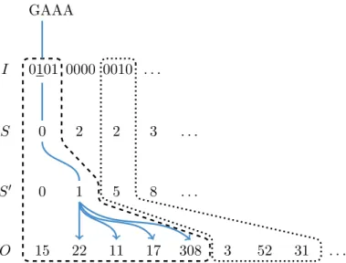
GAAA
I 0101 0000 0010 . . .
S 0 2 2 3 . . .
S0 0 1 5 8 . . .
O 15 22 11 17 308 3 52 31 . . .
Figure 2.1: The q-group index consists of four arraysI, S, S0, O. The dashed and dotted areas show the search spaces in the data structure for q-grams assigned to the first and the third q-group, respectively. The arrows illustrate how the four layers of the index are traversed to reach the occurrences of the queried q-gram GAAA.
Proof. To determine (i, j) such that g = gij, we simply compute i = bg/wc and j = g−wi=gmodwin constant time. To compute the group-rankj0, i.e., find how many one-bits occur up to bit j in I[i], we use the population count instruction with a bit mask
j0 =Popcount(I[i] & (2j−1)).
Given thatw is set to the GPU word size (see above), population counts are available as a hardware instruction. Hence, this needs constant time as well. Thek-th occurrence (starting from zero) of gcan then be calculated as
O[S0[S[i] +j0] +k]
with complexityO(1).
Comparison with rank data structures For a sequence of bits, therank of the k-th bit is the number of 1-bits up to position k. A rank data structure provides the rank for thek-th bit in constant time. Jacobson (1988) calls it succinct, if it needs n+o(n) bits for a bit sequence of length n. The classical succinct rank data structure uses the following strategy (Gonz´alez et al. 2005). The bit sequence is partitioned into equally sized superblocks which are themselves divided into blocks. For each superblock, the rank of the first bit is stored in a table. For each block, the rank of the first bit within the superblock is stored. Finally, the rank of each bit in a block can be computed using
the two tables and either the population count operation or an additional table. Since the tables have to store ranks for fewer bits, properly chosen block sizes render their space requirements sublinear in the number of bits in the sequence. When interpreting I as a sequence of bits, I and S implement a rank data structure, with S[i] +j0 + 1 being the rank of the g-th bit in I for q-gram g with i = bg/wc and j = gmodw. While the implementation is not succinct, a single query needs less table lookups. This is beneficial on the GPU since accessing memory is expensive (see Section 1.3).
2.4.1 Size
We note that both I and S consist of d4q/we words, S0 contains an index for each occurring q-gram and hence of up to min{4q,|T|} words, and O is a permutation of text positions consisting of|T|words. The size of the q-group index follows directly as the sum of its components:
Theorem 2.4. Let T be a text and IT,q := (I, S, S0, O) be the corresponding q-group
index. Then, IT ,q needs up to 24q
w
+ min{4q,|T|}+|T|words.
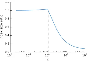
We evaluate how above worst case size of the q-group index behaves compared to the size of the q-gram index (i.e., 4q+|T|; see Section 2.3). Both depend on the size of the underlying text and the value of q, manifesting in the number of possible q-grams 4q. Therefore, we consider the ratioK between the possible q-grams and the text size, i.e., 4q =K|T|. We further assume a word size ofw= 32 bits.
If 4q/|T|, the conventional q-gram index has a small advantage because each q-gram can be expected to occur (even multiple times). With K ≤ 1, the size ratio between q-group index and q-gram index is
2 324 q+ 4q+|T| 4q+|T| = K 16|T|+K|T|+|T| K|T|+|T| = K 16+K+ 1 K+ 1 = 1 + K 16(1 +K).
For K = 1 (or |T| = 4q), this means a small size disadvantage of 3% for the q-group index.
If q becomes larger for fixed text size (such that q-grams become sparse), the q-group index saves memory, up to a factor of 16. The size ratio is
2 324q+|T|+|T| 4q+|T| = K 16|T|+|T|+|T| K|T|+|T| = K 16+ 2 K+ 1
0.0
0.2
0.4
0.6
0.8
1.0
1.2
index size ratio
10
-210
-110
010
110
2K
Figure 2.2: Ratio between the worst case size of the group index and the size of the q-gram index for different K= 4q/|T|. The dashed line marks the break-even point, i.e., theK beyond which the q-group index guarantees to be smaller than the classical q-gram index.
for K > 1 and tends to 161 for large K. The break-even point is reached for K = 1615. Figure 2.2 shows the behavior of the index size ratio depending onK.
In practice, we useq = 16 because of the following reasons. First, a bit-encoded 16-gram exactly fills a 32-bit word and hence avoids wasting bits. Second, todays usual reads contain 100 bases or more and the tendency is to produce rather larger than shorter reads. In this scenarioq = 16 offers reasonable error tolerance and high specificity. With current GPU memory size, we use |T|= 108, i.e., we process 100 million nucleotides at a time. In the worst case, this results in a q-group index size of approximately 1.8 GB. The ratio between q-grams and text size is K= 42.95, and the q-group index needs in the worst case 4242.95.95+1/16+2 ≈10% of the memory of the conventional q-gram index.
2.4.2 Construction
Algorithm 1 shows how the index is built. The outline of the algorithm is as follows. First, I is created from the q-grams of the text (line 2). Then, S is calculated as the cumulative sum over the population counts ofI(line 6). Next, the number of occurrences for each q-gram is calculated (line 10) and S0 is created as the cumulative sum over these counts (line 14). Finally, the q-gram positions are written into the appropriate intervals ofO (line 16).
Each step is implemented on the GPU with parallel OpenCL kernels (see Section 1.3). The cumulative sums are implemented with parallelized prefix scan operations (see Sec-tion 1.3.2). Importantly, the algorithm needs hardly any branching (hence maximizing concurrency) and makes use of coalescence along the reads to minimize memory latency.
Algorithm 1 Building the q-group index. For a q-gram g, the function Group-And-Bit(g) computes (i, j) with group i:=bg/wc and bitj:=gmodw. The functionGroup-Rank(I, i, j) computesj0 :=Popcount(I[i] & (2j−1)), as explained in the text.
Input: a text T, machine word sizew, q-gram sizeq
Output: the q-group index (I, S, S0, O)
1: initializeI withd4q/we zeros
2: forp←0, . . . ,|T| −q in parallel
3: (i, j)←Group-And-Bit(q-gram at position p inT)
4: I[i]j ←1
5: allocateS with space for|I|+ 1 integers
6: fori←0, . . . ,|I| −1 in parallel
7: S[i+ 1]←Popcount(I[i])
8: S← cumulative sum of S
9: initializeS0 of lengthS[|I|] + 1 with zeros 10: forp←0, . . . ,|T| −q in parallel
11: (i, j)←Group-And-Bit(q-gram at position p inT)
12: j0 ←Group-Rank(I, i, j)
13: increment S0[S[i] +j0+ 1] by 1
14: S0← cumulative sum of S0
15: AllocateO of length|T|
16: forp←0, . . . ,|T| −q in parallel
17: (i, j)←Group-And-Bit(q-gram at position p inT)
18: j0 ←Group-Rank(I, i, j)
19: k← next free entry inO after S0[S[i] +j0]
20: O[k]←p
All major data structures are kept in GPU memory. Therefore, between the steps, only constant amounts of data (e.g., a single integer defining the size of an array; see line 9) have to be transferred between the GPU and the host.
Theorem 2.5. For a text T and a machine word size w, Algorithm 1 calculates the
q-group index IT ,q:= (I, S, S0, O) with time complexity
O 1 ρ 4q w + min{4 q,|T|}+|T| + logρ
on a CREW PRAM (Section 1.3.1) withρ processors. If|T|<4q, complexity is
O 1 ρ 4q w +|T| + logρ .
Proof. We first prove the time complexity for the general case. Each initialization of an array A with zeros needs |A|operations. Hence, line 1 and 9 need |I| = 4q/w and
|S0| = min{4q,|T|} operations. The operations in all kernels (lines 2, 6, 10 and 16) need constant time (see Theorem 2.3). Therefore, the kernels needO(|T|) andO(|I|) = O(4q/w) operations. Considering a CREW PRAM with ρ processors and excluding the cumulative sums, we obtain a time complexity O((4q/w+ min{4q,|T|}+|T|)/ρ). A cumulative sum on an array A has time complexity O(|A|/ρ+ logρ) on an EREW PRAM (see Section 1.3.2) and therefore also on a CREW PRAM. Since the cumulative sums (line 8 and 14) are calculated onS andS0, the total time complexity is
O 1 ρ 4q w + min{4 q,|T|}+|T| + logρ . If|T|<4q, the minimum can be eliminated, resulting in
O 1 ρ 4q w +|T| + logρ .
For correctness, we first observe that array I is build correctly by the definition of Group-And-Bit. Any q-gram g not contained in the text T does not occur in the other data structures. It remains to show by induction thatO[S0[S[i] +j0] +k] contains thek-th occurrence1of an arbitrary q-gramgij contained in the textT with group-rank j0 after executing Algorithm 1.
We first consider the smallest q-gram g(0) =gij contained in the text T as basis. Since g(0) is the smallest occurring q-gram,S[i+ 1] is the first nonzero entry inSset in line 7. Therefore, the cumulative sum of S in line 8 yields S[i] = 0. Further, the rank of g(0) isj0 = 0, such that line 13 incrementsS0[1] by 1. The cumulative sum in line 14 yields S0[0] = 0. The last step of the algorithm fills consecutive entries of O beginning with S0[0] = 0 with the occurrence position p. Hence, the k-th occurrence of g(0) is located atO[S0[S[i] +j0] +k] =O[k].
Now, we assume that the algorithm is correct for the n-th smallest q-gram g(n) = ginjn occurring m times in the text with group-rank j
0
n. By induction, we know that O[S0[S[in] +j0n] +m−1] contains the last occurrence of q-gramg(n). Let g(n+1) =gij be the (n+ 1)-th smallest q-gram occurring in the text with group-rankj0. It suffices to show thatS0[S[i] +j0] =S0[S[in] +jn0] +m, which follows directly from the observation that the cumulative sum over S0 may only increase by m between S0[S[in] +jn0] and S0[S[i] +j0], because there is no occurring q-gram between g(n+1) and g(n).
In practice, the memory requirements for the q-group index can be reduced further without changing access (Theorem 2.3) and construction (Theorem 2.5) time com-plexities. By storing every even position of S, the q-group index needs only up to
4q
w
+24wq+ min{4q,|T|}+|T|words. The values of the odd positions iof S can be obtained asS[i−1] +Popcount(I[i−1]) in constant time.
1Note that, in practice, the synchronization between threads when writing ofOdoes not guarantee
that the k-th occurrence in the index is also the k-th occurrence of the q-gram in the text. The sequence of occurences of a q-gram inOis rather a permutation thereof.
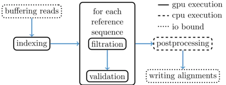
filtration validation for each reference sequence indexing buffering reads postprocessing writing alignments io bound cpu execution gpu execution
Figure 2.3: The PEANUT algorithm. Read sequences are buffered and a q-group index is created from them on the fly. Filtration (detection of q-gram hits) and validation are performed on the GPU until all reference sequences (e.g., chromosomes) are processed. The hits are postprocessed and streamed out in SAM format. All steps (here shown as boxes) operate independently in parallel and communicate via queues. Arrows between the steps represent a data transfer via a queue.
2.5 Algorithm
On top of the q-group index, we define the PEANUT algorithm for read mapping. The algorithm consists of three main steps:
1. filtration, 2. validation, 3. postprocessing.
The first two steps, filtration and validation, are handled on the GPU, while the postpro-cessing is computed on the CPU. The steps are conducted on a stream of reads. Reads are collected until buffers of configurable size are saturated. Then, any computation is done in parallel for all buffered reads (see Figure 2.3).
In the filtration step, potential hits between the reference sequence and the reads are detected using the q-group index. Next, the potential hits are validated using a variant of Myers’ bit-parallel alignment algorithm (Myers 1999). The validated hits undergo a postprocessing that annotates them with a mapping quality and calculates the actual alignment. The postprocessed hits are streamed out in SAM format (Li et al. 2009). Because of memory constraints on the GPU, all steps are performed per reference se-quence (e.g., chromosome) instead of using the reference as a whole (see Section 2.5.1). Paired-end reads (see Section 1.2) are handled independently during filtration and val-idation. During postprocessing, read-pair information is used to sort hits into strata of decreasing confidence and obtain mapping qualities (see Section 2.5.3). In the following, each step is described in detail.
2.5.1 Filtration
For a given subset of reads loaded into the buffer (see above), the filtration step aims to yield a set of potential hits, i.e., candidate origins of each read. For this, we seek for matching q-grams between each reference sequence and the reads using the q-group index (Section 2.4).
Following Weese, Holtgrewe, and Reinert (2012), we decide to build the q-group index over the concatenation of the buffered reads. At first sight, it would be more reasonable to build the index over the reference. However, building the q-group index over the whole reference (i.e., the concatenation of all reference sequences) would exceed the memory of most GPUs, since most q-grams would occur and the size advantage of the q-group index would vanish (see Section 2.4.1). Alternatively the index could be build over parts of the reference (as, e.g., naturally given by the reference sequences). Since not all indexes for all reference sequences could stay in memory, either building them online or loading them from a preprocessed storage would be necessary. Hence, either |R| large data transfers or |R| index builts would have to be repeated for each set of buffered reads and |R| reference sequences. Since the q-group index is per definition larger than the underlying text, it is better to keep the reference sequences in GPU memory and build the index once over the set of buffered reads.
Given the q-group index (I, S, S0, O), we assume that there is a function Indexpair(g) that returns, for a q-gramg, an index pair (kstart, kend) such that the occurrence
posi-tions in the indexed text are allO[k] withkstart ≤k < kend. The functionIndexpair(g)
is implemented as follows. Let (i, j) :=Group-And-Bit(g) and the group-rank j0 := Group-Rank(I, i, j). Thenkstart=S0[S[i] +j0] andkend=S0[S[i] +j0+ 1]. We further
assume thatkstart =kend ifgdoes not occur in the index, i.e., I[i]j = 0.
Algorithm 2 shows how putative hits are generated by querying the q-group index of buffered reads with q-grams of a reference sequence. Instead of considering all positions within the reference sequence, we allow to only use q-grams starting at a given subsetP of reference positions. This allows to omit uninformative regions (see below). First, the number of hits per reference position is counted in parallel and stored in the array C (line 2). In the following, only positions with at least one hit are considered (line 5). The cumulative sum of the counts generates an interval for each position that determines where its hits are stored in the output array of the algorithm (line 6). Finally the occurrences for each reference q-gram are translated into hits that are stored in the corresponding interval of the output array (loop in line 8). We translate the position inside the text of concatenated reads into a read number (line 12) and a “hit diagonal” that denotes the putative start of the read in the reference (line 13, see Figure 2.4). For the read number, we assume that all reads are of the same lengthm. The practical implementation uses padding where this is not the case.
Each step of Algorithm 2 is implemented on the GPU with parallel OpenCL kernels. The filtering of P (line 5) and the cumulative sum (line 6) uses parallel prefix scans
Algorithm 2 Filtration of reference positions.
Input: reference sequence, ordered set P of considered reference positions withpl∈P
being thel-th element of P, maximum read length m, q-group index (I, S, S0, O)
Output: array H of hits as pairs (d, r) of diagonal dand read id r
1: Initialize arrayC of length|P|+ 1 with zeros to count hits
2: forpi ∈P in parallel
3: (kstart, kend)←Indexpair(q-gram at reference position pi)
4: C[l+ 1]←kend−kstart
5: P ← {pl ∈P |C[l+ 1]>0}
6: C← cumulative sum ofC
7: Allocate arrayH of length 2·C[|P|] to store hits
8: forpi ∈P in parallel
9: (kstart, kend)←Indexpair(q-gram at reference position pi)
10: for k←0. . . , kend−kstart−1do
11: p0 ←O[kstart+k]
12: r← bp0/mc
13: d←p−(p0modm)
14: H[C[l] +k]←(d, r)
(see Section 1.3.2). All data structures reside in GPU memory; between the steps, at most constant amounts of data have to be transferred between host and GPU (e.g., a single integer). When fixing the number of PRAM processors, Algorithm 2 has the best possible time complexity, becoming linear in the number of investigated positions and obtained hits:
Theorem 2.6. For a reference sequence with positions P, a q-group index(I, S, S0, O)
over reads of maximum length m and a machine word size w, Algorithm 2 calculates putative hits H between reads and reference sequence with time complexity
O
|
H|+|P|
ρ + logρ
on a CREW PRAM with ρ processors.
Proof. The array initializations in line 1 and 7 need |P|+ 1 and |H| operations. The first parallel kernel (line 2) has time complexityO(|P|/ρ) on the CREW PRAM. The second kernel (line 8) calculates each hit in constant time (see Theorem 2.3) and hence has time complexity O(|H|/ρ) on the PRAM. Finally the position filtering (line 5), implemented using a prefix scan (see Section 1.3.2), and the cumulative sum have time complexityO(|P|/ρ+ logρ), resulting in above total complexity.
For correctness, we show that the resulting array H contains exactly all hits between the reference sequence at positions P and the reads. For the l-th position pl ∈ P, we say that it occurs in the reads if the q-gram starting at positionpl occurs in the reads. Analogously, we say that pl does not occur if the q-gram does not occur in the reads.
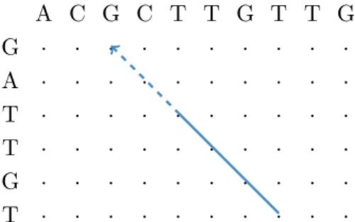
A C G C T T G T T G G · · · · A · · · · T · · · · T · · · · G · · · · T · · · ·
Figure 2.4: Determining the putative start position of a read from a matching q-gram via a hit diagonal (Rasmussen, Stoye, and Myers 2006). In the edit matrix between the reference sequence (top) and the read (left), a matching q-gram (solid line) induces (under the assumption that the read does not contain insertions or deletions before the q-gram) a diagonal that points to a putative start position of the read in the reference (dashed arrow).
We observe that before line 6, C[l+ 1] contains the occurrence counts of the q-gram at the l-th position pl ∈ P by definition of the function Indexpair. Then, it follows directly that the cumulative sum in line 6 results in C[l] to contain the sum of the occurrence counts of positions pl0 ∈ P with l0 < l. Hence, the array H has the same number of entries as there are hits between the reference sequence at positions P and the reads (line 7). It remains to be shown that all hits of occurring positions are written into disjoint entries of H and that no hits are generated from positions that do not occur in the reads.
We first consider the second case: Let pl ∈P be any non-occurring position. We note that C[l+ 1] = 0 because kstart =kend and pl is removed from the set P in line 5. It therefore does not occupy any entries inH.
We prove the other case by induction. As basis, letpl ∈P be the first reference position occurring in the reads. Let m be the number of occurrences of the q-gram starting at position pl. Since pl is the first occurring reference position, it holds C[l] = 0. Hence, the k-th hit (with 0 ≤ k < m) determined from the q-group index is stored in entry H[k] and all m hits are stored inH[0], . . . , H[m−1].
Now, we assume that then-th positionpn∈P occursmntimes in the reads. We consider the (n+ 1)-th position pn+1 ∈ P with mn+1 occurrences. Without loss of generality,
we assume mn>0 and mn+1 >0 (which can always be achieved by reordering the set
P). Since there are no occurring positions in between, the cumulative sum ensures that C[n+ 1] =C[n] +mn. By induction, we know that H[0]. . . H[C[n] +mn−1] are filled with correct hits. Finally, the k-th hit of pn+1 is stored in H[C[n+ 1] +k] such that
H[0], . . . , H[C[n+ 1] +mn+1−1] is correct, too.
starting position by their diagonal (see Figure 2.4). This occurs in regions where the identity between read and reference is high. Instead of reducing these to a single hit, we found it to be faster to validate all hits and perform the removal of duplicates on those remaining after the validation step (see Section 2.5.3).
Reference sequence preprocessing The set P of reference positions to investigate and the reference sequences are retrieved from a precomputed data structure stored in HDF5 format2. First, this speeds up access to the reference. Second, we omit exceedingly frequent q-grams and stretches of unknown nucleotides (i.e., subsequences of Ns, see Section 2.3) from the setP. For q-